Chapter 10 Applications

• Recently published empirical studies using a structural estimation based on a partial equilibrium model, mostly in the field of industrial organization.

10.1 2018-2019

10.1.1 American Economic Review

• Wollmann (2018): Estimate a structural model of the US commercial vehicle market and demonstrate the importance of allowing for endogenous product offerings in a merger analysis.

• Dinerstein, Einav, Levin, & Sundaresan (2018): Study how the redesign of the search engine at eBay affect consumer search and price competition among sellers.

• Crawford, Pavanini, & Schivardi (2018): Estimate a structural model of credit demand, loan use, pricing, and firm default using matched firm-bank data from Italy, and find evidence of adverse selection and how banks can mitigate the negative effects by adjusting credit supply.

• Hortaçsu, Kastl, & Zhang (2018): Estimate a structural model of bidding at the uniform price auctions of US Treasury bills and notes that takes into account informational asymmetries introduced by the bidding system and show that primary dealers have bid-shading ability higher than their willingness-to-pay.

• Aizawa & Kim (2018): Estimate an equilibrium model of Medicare Advantage with advertising allowing rich individual heterogeneity and show that advertising is effective in attracting healthy individuals for are newly eligible for Medicare, contributing to advantageous selection into Medicare Advantage.

• Ulrich Doraszelski, Lewis, & Pakes (2018): Draw on models of fictitious play and adaptive learning to analyze the evolution of the new market for frequency response within the UK electricity system and explain the convergence of pricing to a rest point that is consistent with equilibrium play.

• Acemoglu, Akcigit, Alp, Bloom, & Kerr (2018): Estimate a model of firm-level innovation, productivity growth, and reallocation featuring endogenous entry and exit and the selection between high- and low-type firms which differ in terms for their innovation capacity, and show that taxing the continued operation of incumbent can lead to gains because of the exit of less productive firms.

• Dubois & Lasio (2018): Estimate a structural model of pharmaceutical with price constraints and infer whether these constraints are binding and study its consequences.

• Ho & Lee (2019): Estimate a Nash-in-Nash bargaining model between insurers and hospitals and evaluate the consequence of narrowing hospital networks in commercial heal care markets in the US.

• Crawford, Shcherbakov, & Shum (2019): Estimate a model of endogenous quality choice in imperfectly competitive markets and show that a quality over-provision in the US cable television markets is caused by the presence of competition from high-end satellite TV providers.

• Fack, Grenet, & He (2019): Propose a new approach to estimate student preferences with data from matching mechanisms and estimate the model with school choice data in Paris.

10.1.2 Econometrica

• Trebbi & Weese (2019): Propose methodologies for the detection of unobserved coalitions of militants in conflict areas and apply to the Afghan conflict during the 2004-2009 period and to Pakistan during the 2008-2011 period, identifying systematically different coalition structures.

• Einav, Finkelstein, & Mahoney (2018): Estimate a dynamic discrete choice model of long-term care hospitals discharge decisions and study the design of provider incentive in the post-acute setting.

• Miravete, Seim, & Thurk (2018): Estimate a model of taxation in a imperfectly competitive market that leads to incomplete tax pass-through using a data from alcoholic beverages in Pennsylvania and study the welfare implication of the state’s current tax policy.

• Crawford, Lee, Whinston, & Yurukoglu (2018): Estimate a structural model of view-ship, subscription, distributor pricing, and affiliate fee bargaining using a data set on the US cable an satellite television industry to analyze the impact of simulated vertical mergers and divestitures of regional sports networks on competition and welfare.

• Agarwal & Somaini (2018): Propose an empirical method for studying random utility models in a school choice mechanisms and apply it to the data from Cambridge.

10.2 Asymmetric Information and Market Power

• I present this paper in detail because the structure of the paper, especially the structure of the introduction, is textbook-perfect.
• It also applies textbook-perfect demand and cost estimation techniques but to an empirically interesting setting.
• The introduction consists of:
  • Background and motivation: Following the seminal work…; Although the basic…; The vast majority…; A recent strand…;
  • Question: We measure…
  • Materials: We exploit detailed data on…
  • Methods: After providing reduced-form evidence…
  • Details of the materials and methods: model (We begin by…), its characterization (The degree of competition…), estimation (We estimate the model…), identification (We face two important challenges…).
  • Results: In our results…
  • Counterfactuals: We run three counterfactuals…
  • Implications: All in all…
  • Contributions: Our paper is related to…
• These topics should be discussed in this order in a structural estimation paper.
• The paper is organized as follows:
  • Data: Source; sampling procedure; cleaning; transformation; summary statistics; motivating findings.
  • Model: Economic model to estimate; relevance to the research question; justification of the assumptions; discussion on key channels; relevance to theoretical models in the literature.
  • Estimation: Econometric specification; estimation procedure; identification.
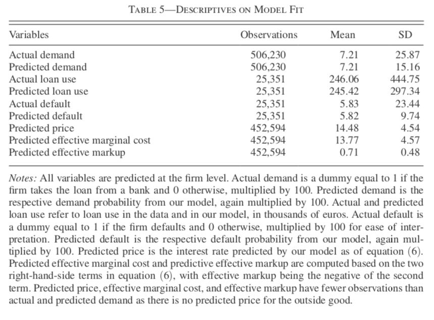
  • Results: Estimation results; key findings and their interpretations; fit of the model.
  • Conterfactuals: Policy experiments; policy implications.
• The data section can come after model and estimation sections if it is a methodological paper that builds estimation and/or identification techniques on an abstract model.

10.2.1 Motivation

• Asymmetric information works differently in imperfectly competitive markets.
• Competitive market: adverse selection \(\to\) higher average cost \(\to\) higher price.
• Imperfectly competitive market: additional channel: adverse selection \(\to\) lower benefit of setting a high price \(\to\) lower price (Lester, Shourideh, Venkateswaran, & Zetlin-Jones, 2018; Mahoney & Weyl, 2017).
• Adverse selection can moderate the welfare losses from market power, and vice versa.

10.2.2 Question, Method, and Materials

• This paper measures the consequences of asymmetric information and imperfect competition in the market for small business lines of credit.
• To do so, formulate and estimate a model of credit demand, loan use, default, and bank pricing;
• using data on a representative sample of Italian firms, the population of medium and large Italian banks, individual lines of credits between them, and subsequent defaults.

10.2.3 Findings

• Find evidence of adverse selection:
  • The unobserved determinants of the choice to borrow and of default are positively correlated.
  • The unobserved determinants of loan use and default are positively correlated.
  • Both are statistically significant.
• Find positive effect of interest rates on default:
  • Evidence of moral hazard?

10.2.4 Policy Experiments

• What if the degree of adverse selection changes?
  • The severer adverse selection still causes a higher price and a smaller credit supply.
  • But market power significantly mitigates this effect.
• What if banks’ cost of capital, say, due to a financial crisis?
  • In the presence of adverse selection, the pass-through is smaller for a bank with higher market power.
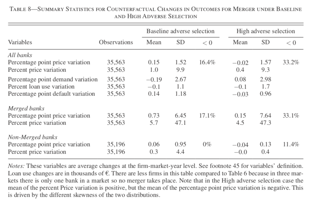
• What if banks merge?
  • Under high adverse selection, a merger can decrease prices.

10.2.5 Source

• Data on individual loans from the Central Credit Register.
• Firm-level balance sheet data from the Company Accounts Data Services.
• Banks’ balance-sheet and income-statement data from the Banking Supervision Register.
• Data on bank branches at the local level.
• The resulting data is over 1988-1998.

10.2.6 Loan Data

• Italian banks have to report data for each individual borrower to the register.
• Focus on the short-term lines of credit:
  • Interest rate is independent of the maturity.
  • Homogeneous product.
  • Not collateralized.
  • Main source of borrowing for Italian firms.
• Focus on firms’ main credit line in the first year they open any credit line.
  • Avoid heterogeneous experience in ratings, loan negotiations, and learning across banks and firms.
• This reduces the sample size from 90,000 to 36,500.
• Average loan amount EUR370,000, average interest rate 14.2%.
• Average bank asset EUR11 billion, average employees 3,200.

10.2.7 Firm Data

• The service collects yearly data on the balance sheets and income statements of a sample of 35,000 Italian non-financial and non-agricultural firms, roughly 30% of the total value added reported in the national accounting.
• The service also computes an indicator of the risk profile of each firm, Score, and reports to banks.
• The Score is approximately the information that a lending bank has available at the time a loan is granted.
• A firm is classified as a borrowing firm if it appears in the Credit Register, and is classified as a non-borrowing firm if it does not appear in the Credit Register and reports zero bank borrowing in the balance sheet.
• Banks’ loan approval decisions are not observed.

10.2.8 Default Data

• A loan is classified as default if a firm’s main line of credit defined it as a bad debt within three years of being granted.
• Reporting a loan as a bad debt to the Credit Registry can happen prior to a legally certified bankruptcy filing, but it usually prevents the firm from borrowing any other loans.
• 6% of new loans default during the sample period.

10.2.9 Positive Correlation Tests

• Positive correlation tests (Chiappori & Salanie, 2000) are often used to test the presence of asymmetric information.
• Are firms more likely to demand credit more likely to default? \[ d_i = 1\{X_i^d \beta + \nu_i > 0\}, \] \[ f_i = \begin{cases} X_i^f \gamma + \eta_i &\text{ if } d_i = 1\\ -&\text{ if } d_i = 0, \end{cases} \] where \(d_i\) is equal to one if the firm borrows and \(f_i\) is equal to one if the borrow defaults.
• \(X_i^d\) and \(X_i^f\) include year, market, firms’ Score, amount of granted credit, sector Fixed effects, firms’ balance sheet variables.
• The number of banks in a firm’s market is only included in \(X_i^d\) (instrument).
• \(f_i\) is observed only if \(d_i = 1\).
• A positive and significant correlation of 0.09 between \(\nu_i\) and \(\eta_i\).
• Are riskier firms use more credit? \[ l_i = X_i \beta + \epsilon_i, \] \[ f_i = X_i \gamma + \eta_i, \] where \(l_i\) is the amount of its loan used by the firm.
• A positive and significant correlation of 0.03 between \(\epsilon_i\) and \(\eta_i\).
• These positive correlations can be interpreted as evidence of adverse selection (Stiglitz & Weiss, 1981).
• We further control several factors such as strategic interactions in the following structural model.

10.2.10 Setting

• Each of \(i = 1, \cdots, I_{mt}\) firms in market \(m\) in year \(t\) is willing to invest in a project and is looking for credit to finance it.
• Firms select their main line of credit from \(j = 1, \cdots, J_{mt}\) banks in \(m\) in \(t\).
• Each bank sets interest rates \(P_{ijmt}\).
• Informational asymmetry: conditional on observable, a firm’s riskiness is known by that firm but not by any of the banks in its market; instead, banks are assumed to known the distribution.
• Screening device: assume that banks use interest rates as their only screening device; the amount of credit granted from a bank to a firm is exogenously given.

10.2.11 Firm Preference over Banks

• Firm \(i\) in market \(m\) in year \(t\) obtains the following utility as it chooses bank \(j\) as its main credit line: \[\begin{equation} U_{ijmt}^D := \overline{\alpha}_0^D + X_{jmt}^{\prime D} \beta^D + \xi_{jmt}^D + \alpha^D P_{ijmt} + Y_{ijmt}^{\prime D} \eta^D + \epsilon_i^D + \nu_{ijmt}^D. \tag{10.1} \end{equation}\]
• \(X_{ijm}^D\): a vector of bank-market-year determinants of demand; observed by everyone.
• \(Y_{ijmt}^D\): a vector of firm-bank-market-year determinants of demand; observed by everyone.
• \(\xi_{jmt}^D\): the bank’s attributes; not observed to econometrician.
• \(\epsilon_i^D\): the firm’s propensity to borrow; only observed to the firm.
• \(\nu_{ijmt}^D\): an idiosyncratic shock; only observed to the firm.
• \(\epsilon_i^D\) is the source of asymmetric information.
• Let \(\alpha_{0i}^D := \overline{\alpha}_0^D + \epsilon_i^D\).

10.2.12 Required Loand Amount

• Firm \(i\) in market \(m\) in year \(t\) borrows the following amount of loan if it chooses bank \(j\) as its main line: \[ L_{ijmt} := \alpha_0^L + X_{jmt}^{\prime L} \beta^L + \alpha^L P_{ijmt} + Y_{ijmt}^{\prime L} \eta^L + \epsilon_i^L. \]
• \(\epsilon_i^L\): the firm’s propensity to use credit; only observed to the firm.
• \(\epsilon_i^L\) is another source of asymmetric information.
• Notice that there is no firm-bank-specific unobserved heterogeneity; why?; we need to know how much a firm will borrow when the firm borrowed from a different bank than in the data; because a loan between a firm and a bank is observed only when the firm borrows from the bank, we need to exclude any firm-bank-specific unobserved heterogeneity in order to predict loans with hypothetical banks.

10.2.13 Default Decision

• Conditional on borrowing, each firm chooses to default if its utility from doing so is greater than 0: \[ U_{ijmt}^F := \alpha_0^F + X_{jmt}^{\prime F} \beta^F + \alpha^F P_{ijmt} + Y_{ijmt}^{\prime F} \eta^F + \epsilon_i^F. \]
• \(\epsilon_i^F\): the firm’s propensity to default; only observed to the firm.
• \(\epsilon_i^F\) is another source of asymmetric information.
• Notice that there is no firm-bank-specific unobserved heterogeneity for the same reason.

10.2.14 Information Structure

• \(\epsilon_i^D, \epsilon_i^L\), and \(\epsilon_i^F\) are assumed to be fixed at the firm level and do not vary across banks.
• They are assumed to follow: \[ \begin{pmatrix} \epsilon_i^D\\ \epsilon_i^L\\ \epsilon_i^F \end{pmatrix} \sim N \left( \begin{pmatrix} 0 \\ 0 \\ 0 \end{pmatrix}, \begin{pmatrix} \sigma_D^2 & \rho_{DL} \sigma_D \sigma_L & \rho_{DF} \sigma_D\\ \rho_{DL} \sigma_D \sigma_L & \sigma_L^2 & \rho_{LF} \sigma_L\\ \rho_{DF} \sigma_D & \rho_{LF} \sigma_L & 1 \end{pmatrix} \right). \]

10.2.15 Moral Hazard

• The model allows for the presence of moral hazard.
• Holmstrom & Tirole (1997): If moral hazard is present, higher repayment requirements on loans can reduce the incentives to exert efforts and increases the default probability.
• Interpreting \(\alpha^F\) a causal effect of price on default (by using an instrument), we will be able to interpret the positive \(\alpha^F\) as evidence of moral hazard.

10.2.16 Bank Problem

• The expected profit for bank \(j\) from charging a price \(P_{ijmt}\) offered to firm \(i\) in market \(m\) in year \(t\) is: \[ \Pi_{ijmt} := P_{ijmt} Q_{ijmt} (1 - F_{ijmt}) - MC_{ijmt} Q_{ijmt}. \]
• \(Q_{ijmt}\): the bank’s expectation of the firm’s demand.
• \(F_{ijmt}\): the bank’s expectation of the firm’s default.
• \(MC_{ijmt}\): the bank’s marginal cost.

10.2.17 The Effect of Price on Default Probability

• There are two channels.
• If \(\alpha^F\) is positive, higher interest rate can increase the default probability, possibly because of moral hazard.
• A higher interest rate also changes the composition of borrower types; borrowing conditional on a high interest rate means that the firm has higher demand for loan; if \(\rho_{DF} > 0\), this implies the firm is riskier.

10.2.18 The First-Order Condition

• The pricing equation is: \[ P_{ijmt} = \frac{MC_{ijmt}}{1 - F_{ijmt} + F_{ijmt}' \mathcal{M}_{ijmt}} + \frac{(1 - F_{ijmt}) \mathcal{M}_{ijmt}}{1 - F_{ijmt} + F_{ijmt}' \mathcal{M}_{ijmt}}. \]
• The first term is the effective marginal cost and the second effective markup.
• \(\mathcal{M}_{ijmt} := - Q_{ijmt} / Q_{ijmt}'\) is the bank \(j\)’s markup on a loan to firm \(i\).

10.2.19 The Effect of Higher Adverse Selection

• As measured by the higher \(\rho_{DF}\).
• Average borrower effect: tends to increase the price.
  • A higher \(\rho_{DF}\) implies a higher default probability \(F_{ijmt}\) for a given price.
  • This decreases the denominator of the pricing equation.
• Marginal borrower effect: tends to suppress the price.
  • A higher \(\rho_{DF}\) (in most cases) implies a higher sensitivity of default probability to price \(F_{ijmt}'\) for a given price.
  • This increases the denominator of the pricing equation.
  • Because the marginal borrower is safer than the average borrow to larger degree, the firm will want to keep them by reducing the price.
• Which of the effects dominates depend on the markup \(\mathcal{M}_{ijmt}\).
  • Low levels of competition imply margins are high, increasing the value to the bank of marginal borrowers.

10.2.20 Estimating Equilibrium Pricing Strategy and Augmenting Missing Price Data

• To estimate bank choice problem for a firm, we need to have price for each pair of bank and firm.
• However, the price is observed only between a bank and a firm that actually held a credit line.
• We augment the missing price by predicted values.
• But the prediction depends on what kind of information set we assume for banks’ pricing decisions.
• We assume that large banks mostly predict the demand based on hard information such as the balance-sheet and income-statement variables and Scores.
• Specifically, we fit the following model to observed prices: \[ P_{ijmt} = \gamma_0 + \gamma_1 \mathcal{D}_{ijmt} + \gamma_2 \mathcal{L}_{ijmt} + \lambda_{jmt} + \omega_i^P + \tau_{ijmt}. \]
• \(\mathcal{D}_{ijmt}\) is the distance between firm \(i\) and the nearest branch of bank \(j\).
• \(\mathcal{L}_{ijmt}\) are dummies for the size of the granted loan amount.
• Regard this as a reduced-form estimates of the equilibrium pricing strategy of the banks.
• Let \(\tilde{\gamma}_0\), \(\tilde{\gamma}_1\), \(\tilde{\gamma}_2\), \(\tilde{lambda}_{jmt}\), and \(\tilde{\omega}_i^P\) the estimates.
• Let \(\tilde{P}_{ijmt}\) be the predicted value from these estimates: \[\begin{equation} \begin{split} \tilde{P}_{ijmt} &:= \tilde{\gamma}_0 + \tilde{\gamma}_1 \mathcal{D}_{ijmt} + \tilde{\gamma_2} \mathcal{L}_{ijmt} + \tilde{\lambda}_{jmt} + \tilde{\omega}_i^P\\ &:= \tilde{P}_{jmt} + \tilde{\gamma}_1 \mathcal{D}_{ijmt} + \tilde{\gamma_2} \mathcal{L}_{ijmt} + \tilde{\omega}_i^P. \end{split} \tag{10.2} \end{equation}\]
• We predict prices offered to non-borrowing firms by propensity score matching.

10.2.21 Inserting Pricing Estimates into the Utility

• We assume that firm-bank-market-year determinants of demand \(Y_{ijmt}^D\) is of the following form: \[ Y_{ijmt}^D := \eta_1^D \mathcal{D}_{ijmt} + \eta_2^D \mathcal{L}_{ijmt} + \eta_3^D Y_i + \omega_i^D. \]
• \(Y_i\) is the observed firm covariates.
• \(\omega_i^D\)$ is the firm covariates not observed to econometrician.
• We further assume that unobserved firm-level attributes \(\omega_i^D\) determining the demand is related to unobserved firm-level attributes \(\omega_i^P\) determining bank’s pricing decision are related as: \[ \omega_i^D = \eta_4^D \omega_i^P. \]
• Because previous regression of price gives estimates of \(\omega_i^P\), \(\tilde{\omega}_i^P\), we treat this as if an observed covariate.
• At the end, we have: \[\begin{equation} Y_{ijmt}^{\prime D} \eta^D = \eta_1^D \mathcal{D}_{ijmt} + \eta_2^D \mathcal{L}_{ijmt} + \eta_3^D Y_i + \eta_4 \tilde{\omega_i}^P. \tag{10.3} \end{equation}\]
• Inserting equations (10.2) and (10.3) into equation (10.1) gives us: \[\begin{equation} \begin{split} U_{ijmt}^D &= \overline{\alpha}_0^D + X_{jmt}^{\prime D} \beta^D + \xi_{jmt}^D + \alpha^D P_{ijmt} + Y_{ijmt}^{\prime D} \eta^D + \epsilon_i^D + \nu_{ijmt}^D\\ &= \overline{\alpha}_0^D + X_{jmt}^{\prime D} \beta^D + \xi_{jmt}^D + \alpha^D[\tilde{P}_{jmt} + \tilde{\gamma}_1 \mathcal{D}_{ijmt} + \tilde{\gamma_2} \mathcal{L}_{ijmt} + \tilde{\omega}_i^P] + \eta_1^D \mathcal{D}_{ijmt} + \eta_2^D \mathcal{L}_{ijmt} + \eta_3^D Y_i + \tilde{\omega}_i^D\\ &= \underbrace{(\overline{\alpha}_0^D + X_{jmt}^{\prime D} \beta^D + \xi_{jmt}^D + \alpha^D \tilde{P}_{jmt})}_{\tilde{\delta}_{jmt}^D} + \underbrace{(\eta_1^D + \alpha^D \tilde{\gamma}_1)}_{\tilde{\eta}_1^D}\mathcal{D}_{ijmt} + \tilde{(\eta_2^D + \alpha^D \tilde{\gamma}_2^D)}_{\tilde{\eta}_2^D} \mathcal{L}_{ijmt}\\ &+ \eta_3^D Y_i + \underbrace{(\eta_4^D + \alpha^D)}_{\tilde{\eta}_4^D} \tilde{\omega}_i^P + \epsilon_i^D + \alpha^D \underbrace{\tilde{\tau}_{ijmt} + \nu_{ijmt}}_{\zeta_{ijmt}}\\ &:= \tilde{\delta}_{jmt}^D + Y_{ijmt}^{\prime D} \tilde{\eta}^D + \epsilon_i^D + \zeta_{ijmt}\\ &:= \tilde{\delta}_{jmt}^D(X_{jmt}^D, \widetilde{P}_{jmt}, \xi_{jmt}^D, \overline{\alpha}_0^D, \alpha^D, \beta^D) + V_{ijmt}^D(Y_{ijmt}^D, \sigma_D, \tilde{\eta}^D) + \zeta_{ijmt}. \end{split} \end{equation}\]
• \(Y_{ijmt}^D : = \{\mathcal{D}_{ijmt}, \mathcal{L}_{ijmt}, Y_i, \tilde{\omega}_i^P\}\).
• \(\tilde{\eta}^D := \{\tilde{\eta}_1^D, \tilde{\eta}_2^D, \eta_3^D, \tilde{\eta}_4^D\}\).
• Inserting the reduced-form estimates of the equilibrium pricing strategy into the demand model; kind of CCP approach; find parameters that make this estimate consistent with equilibrium conditions.
• Predictors for the equilibrium pricing strategy is all included in the utility for choosing a bank; thus, at the equilibrium, the change in covariate affect the utility through two channels; direct effect and indirect effect through price change; \(\tilde{\eta}_1^D, \tilde{\eta}_2^D\), and \(\tilde{\eta}_4^D\) represent the composite effects; because the effect on pricing is already identified, we can separate the effects through these two channels in the second stage.
• The error terms is also a composite of preference shock \(\nu_{ijmt}\) and prediction error in pricing \(\tilde{\tau}_{ijmt}\).
• \(\alpha_D\) is identified in the second stage after estimating \(\tilde{\eta}^D\) in the first stage.

10.2.22 Choice Probability

• The probability that borrower \(i\) in market \(m\) in year \(t\) chooses bank \(j\) is given by: \[ Pr_{ijmt}^D := \int \frac{\exp[\tilde{\delta}_{jmt}^D(X_{jmt}^D, \widetilde{P}_{jmt}, \xi_{jmt}^D, \overline{\alpha}_0^D, \alpha^D, \beta^D) + V_{ijmt}^D(Y_{ijmt}^D, \sigma_D, \tilde{\eta}^D)]}{1 + \sum_{l} \exp[\tilde{\delta}_{lmt}^D(X_{lmt}^D, \widetilde{P}_{lmt}, \xi_{lmt}^D, \overline{\alpha}_0^D, \alpha^D, \beta^D) + V_{ilmt}^D(Y_{ilmt}^D, \sigma_D, \tilde{\eta}^D)]} f(\epsilon_i^D) d\epsilon_i^D. \]

10.2.23 Equilibrium Loan Strategy

• In the equilibrium, the probability of having loan \(L\) conditional on borrowing (\(D = 1\)) is: \[\begin{equation} \begin{split} Pr_{ijmt, L|D = 1}^L &:= \mathbb{E}\left\{\mathbb{P}[L_{ijmt} = \alpha_0^L + \alpha^L P_{ijmt} + Y_{ijmt}^{\prime L} \eta^L + \epsilon_i^L|\epsilon_i^D] D = 1 \right\}\\ &= \int \phi_{\epsilon_i^L|\epsilon_i^D} \left(\frac{L_{ijmt} - \alpha_0^L - \alpha^L P_{ijmt} - Y_{ijmt}^{\prime L} \eta^L - \tilde{\mu}_{\epsilon_i^L|\epsilon_i^D}^L}{\tilde{\sigma}_{\epsilon_i^L|\epsilon_i^D}} \right) f(\epsilon_i^D|D = 1) d \epsilon_i^D. \end{split} \tag{10.4} \end{equation}\] where \[ \epsilon_i^L | \epsilon_i^D \sim N\left(\frac{\sigma_L}{\sigma_D} \rho_{DL} \epsilon_i^D, \sigma_L^2 (1 - \rho_{DL}^2) \right) := N(\tilde{\mu}_{\epsilon_i^L|\epsilon_i^D}^, \tilde{\sigma}_{\epsilon_i^L|\epsilon_i^D}). \]

10.2.24 Equilibrium Default Strategy

• In the equilibrium, the probability of default (\(F = 1\)) conditional on borrowing (\(D = 1\)) is: \[\begin{equation} \begin{split} Pr_{ijmt, F = 1| D = 1, L}^F &:= \int \Phi_{\epsilon_i^F|\epsilon_i^D, \epsilon_i^L}\left(\frac{\alpha_0^F + X_{jmt}^{\prime F} \beta^F + \alpha^F P_{ijmt} + Y_{ijmt}^{\prime F} \eta^F - \tilde{\mu}_{\epsilon_i^F|\epsilon_i^D, \epsilon_i^L}}{\tilde{\sigma}_{\epsilon_i^F | \epsilon_i^D, \epsilon_i^L}} \right) f(\epsilon_i^D | D = 1) d\epsilon_i^D, \end{split} \tag{10.5} \end{equation}\] where \[ \epsilon_i^F | \epsilon_i^D, \epsilon_i^L \sim N(A \epsilon_i^D + B \epsilon_i^L, \sigma_F^2 - (A \rho_{DF} + B \rho_{LF})) := N(\tilde{\mu}_{\epsilon_i^F|\epsilon_i^D, \epsilon_i^L}, \tilde{\sigma}_{\epsilon_i^F | \epsilon_i^D, \epsilon_i^L}). \] \[ A := \frac{\rho_{DF} \sigma_L^2 - \rho_{LF} \rho_{DL}}{\sigma_D^2 \sigma_L^2 - \rho_{DL}^2}. \] \[ B := \frac{-\rho_{DF} \rho_{DL} + \rho_{LF} \sigma_D^2}{\sigma_D^2 \sigma_L^2 - \rho_{DL}^2}. \]

10.2.25 Control Function Approach to Deal with Endogeneity in Loand and Defaulty Equations

• The structural parameters in loan use and default strategies are identified by using instrumental variables.
• Use prices in the other market as instruments (Hausman-type instruments).
• Use a control function approach.
• Regress prices on the convariates in loan use equation and the instrument.
• Let \(\hat{u}_{ijmt}^L\) be the residual estimate.
• Regress prices on the covariates in default equation and the instrument.
• Let \(\hat{u}_{ijmt}^F\) be the residual estimate.
• Replace \(\tilde{P}_{jmt}\) in equation (10.4) with the predicted value plus \(\hat{u}_{ijmt}^L\).
• Replace \(\tilde{P}_{jmt}\) in equation (10.5) with the predicted value plus \(\hat{u}_{ijmt}^F\).
• Because of the instruments, the values of \(\hat{u}_{ijmt}^L\) and \(\hat{u}_{ijmt}^F\) can change conditional on the covariates in the loan strategy and default strategy.
• These variations identify \(\alpha^L\) and \(\alpha^F\) in the following first-stage equation.

10.2.26 First-Stage Estimation

• In the first-stage, we identify the composite parameters in the bank choice; the coefficients consist of structural parameters and the biases from endogeneity.
• We separate structural parameters from biases in the second stage using instrumental variables.
• We estimate parameters by maximizing the following simulated log-likelihood function: \[ log L := \sum_{i} d_{ijmt} \{\log(P_{ijmt}^D) + \log (Pr_{immt}^L) + f_{ijmt} \log (Pr_{ijmt}^T) + (1 - f_{ijmt}) log (1 - Pr_{ijmt}^F) \}. \]
• \(d_{ijmt}\): firm \(i\) borrows from bank \(j\) in market \(m\) in year \(t\).
• \(f_{ijmt}\): firm \(i\) defaults from bank \(j\)

10.2.27 Second-Stage Estimation

• From the first-stage estimates, we obtain the estimate of \(\tilde{\delta}_{jmt}\), denoted by \(\hat{\tilde{\delta}_{jmt}}\).
• Consider a regression such as: \[ \hat{\tilde{\delta}_{jmt}} = \overline{\alpha}_0^D + \alpha^D \tilde{P}_{jmt} + X_{jmt}^{\prime D} \beta^D + \xi_{jmt}^D, \] where \(\tilde{P}_{jmt}\) and \(\xi_{jmt}^D\) can be correlated.
• Use the euro value of collected deposits and the number of deposit accounts at the bank-market-year level as instruments.
• The high degree of autonomy that local branch managers have in their lending decisions will imply better service and condition for loans.
• Because deposit conditions are determined in the market with households, it will be independent of loan market conditions.

10.2.28 Estimation Results

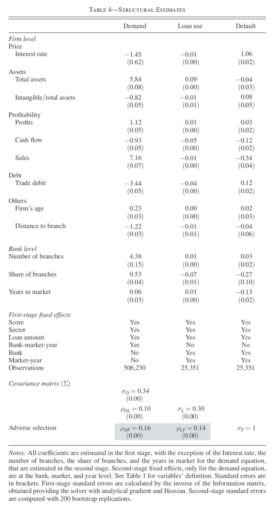
10.2.29 Findings from Estimation Results

• Interest rates have negative impact on bank choice and loan amount.
  • On average among five largest banks, 10% increase in the interest rate reduces the bank’s market share by 10% and increases rival banks’ shares by 1%.
• A higher interest rate leads to a higher default probability.
  • If the control function approach successfully identify the structural effect of price increase on the default probability, the positive estimate can be interpreted as evidence of moral hazard as we have discussed.
• Correlation between unobserved demand and loan amount shocks, and between demand and default shocks, are positive and statistically significant.

10.2.30 Fit of the Model

10.2.31 Counterfactuals

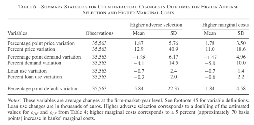
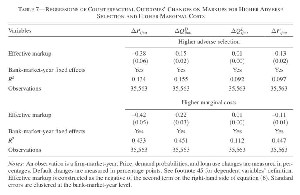
10.2.32 What if Adverse Selection Got Severer?

• A doubling in the correlations \(\rho_{DF}\) and \(\rho_{LF}\) causes 1.87 percent points increases in the average interest rates.
• This causes 1.28 percent points decrease in the share and EUR700 decrease in the loan amount.
• The default probability substantially increases from 5.5 to 11.4%.
• The effective markup of a bank is negatively correlated with the price and default probability changes, and positively correlated with demand and loan amount changes.
  • A bank with higher market power takes care of marginal borrowers more than a bank with less market power.

10.2.33 What if Cost of Capital Increased?

• 5% (or 70 basis points) increase in the bank’s marginal cost leads to 1.78 percent points increase in the interest rates.
• The default probability increases only by 1.84 percent points in this case.
  • With price increase, riskier borrowers will borrow from a bank.
  • But in the current case, the degree of adverse selection is fixed.
  • So the increase in default probability is moderate.
• The effective markup of a bank is negatively correlated with the price and default changes, and positively correlated with demand and loan amount change.

10.2.34 Merger Simulation

• Under severe adverse selection, unilateral effects of a merger on prices is moderate.

References

Acemoglu, D., Akcigit, U., Alp, H., Bloom, N., & Kerr, W. (2018). Innovation, Reallocation, and Growth. American Economic Review, 108(11), 3450–3491.

Agarwal, N., & Somaini, P. (2018). Demand Analysis Using Strategic Reports: An Application to a School Choice Mechanism. Econometrica, 86(2), 391–444.

Aizawa, N., & Kim, Y. S. (2018). Advertising and Risk Selection in Health Insurance Markets. American Economic Review, 108(3), 828–867.

Chiappori, P.-A., & Salanie, B. (2000). Testing for Asymmetric Information in Insurance Markets. Journal of Political Economy, 108(1), 56–78.

Crawford, G. S., Lee, R. S., Whinston, M. D., & Yurukoglu, A. (2018). The Welfare Effects of Vertical Integration in Multichannel Television Markets. Econometrica, 86(3), 891–954.

Crawford, G. S., Pavanini, N., & Schivardi, F. (2018). Asymmetric Information and Imperfect Competition in Lending Markets. American Economic Review, 108(7), 1659–1701.

Crawford, G. S., Shcherbakov, O., & Shum, M. (2019). Quality Overprovision in Cable Television Markets. American Economic Review, 109(3), 956–995.

Dinerstein, M., Einav, L., Levin, J., & Sundaresan, N. (2018). Consumer Price Search and Platform Design in Internet Commerce. American Economic Review, 108(7), 1820–1859.

Doraszelski, Ulrich, Lewis, G., & Pakes, A. (2018). Just Starting Out: Learning and Equilibrium in a New Market. American Economic Review, 108(3), 565–615.

Dubois, P., & Lasio, L. (2018). Identifying Industry Margins with Price Constraints: Structural Estimation on Pharmaceuticals. American Economic Review, 108(12), 3685–3724.

Einav, L., Finkelstein, A., & Mahoney, N. (2018). Provider Incentives and Healthcare Costs: Evidence From Long-Term Care Hospitals. Econometrica, 86(6), 2161–2219.

Fack, G., Grenet, J., & He, Y. (2019). Beyond Truth-Telling: Preference Estimation with Centralized School Choice and College Admissions. American Economic Review, 109(4), 1486–1529.

Ho, K., & Lee, R. S. (2019). Equilibrium Provider Networks: Bargaining and Exclusion in Health Care Markets. American Economic Review, 109(2), 473–522.

Holmstrom, B., & Tirole, J. (1997). Financial Intermediation, Loanable Funds, and The Real Sector. The Quarterly Journal of Economics, 112(3), 663–691.

Hortaçsu, A., Kastl, J., & Zhang, A. (2018). Bid Shading and Bidder Surplus in the US Treasury Auction System. American Economic Review, 108(1), 147–169.

Lester, B., Shourideh, A., Venkateswaran, V., & Zetlin-Jones, A. (2018). Screening and Adverse Selection in Frictional Markets. Journal of Political Economy, 127(1), 338–377.

Mahoney, N., & Weyl, E. G. (2017). Imperfect Competition in Selection Markets. The Review of Economics and Statistics, 99(4), 637–651.

Miravete, E. J., Seim, K., & Thurk, J. (2018). Market Power and the Laffer Curve. Econometrica, 86(5), 1651–1687.

Stiglitz, J. E., & Weiss, A. (1981). Credit Rationing in Markets with Imperfect Information. The American Economic Review, 71(3), 393–410.

Trebbi, F., & Weese, E. (2019). Insurgency and Small Wars: Estimation of Unobserved Coalition Structures. Econometrica, 87(2), 463–496.

Wollmann, T. G. (2018). Trucks without Bailouts: Equilibrium Product Characteristics for Commercial Vehicles. American Economic Review, 108(6), 1364–1406.