Chapter 5 Merger Analysis
5.1 Motivations
- Measuring the market power of firms and predicting the possible consequence of horizontal merger cases is one of the primary goal of empirical industrial organization.
- This is important for antitrust authority to review merger cases.
- To do so, we integrate the product/cost function estimation and demand function estimation techniques.
- We introduce the last piece of parameters that characterize the market competition, conduct parameter, and discuss its identification.
- Then, we conduct the first kind of counterfactual analysis, the merger simularion.
- In this exercise, we predict the market response when the ownership structure of product is changed due to a hypothetical merger.
- Every market institution needs its own model for merger simulation:
- Gowrisankaran, Nevo, & Town (2015):
- In the U.S. hospitals and managed care organizations (MGO) negotiate the hospital prices and the coinsurance rates.
- What if hospitals are merged? How much do the hospital prices and the coinsurance rates increase?
- Smith (2004):
- Sometimes the same service is sold through multiple stores such as in the supermarket industry.
- How does this multi-store nature affect the merger effects?
- Ivaldi & Verboven (2005) reviews the cases in the European Commission.
5.2 Identification of Conduct
5.2.1 Identification of Conduct
- So far we have been concerned with the two types of parameters:
- Production and/or cost function.
- Demand function.
- To identify the marginal cost by the revealed preference approach, we have assumed that firms are engaging in a price competition.
- The mode of competition is another parameter of interest.
- Can we infer the mode of competition instead of assuming it?
5.2.2 Marginal Revenue Function
- To be specific, consider firms producing homogeneous product.
- Under what conditions can we distinguish across Bertrand competition, Cournot competition, and collusion? (Timothy F. Bresnahan, 1982).
- Consider the following marginal revenue function: \[\begin{equation} MR(Q) \equiv \lambda Q P'(Q) + P(Q), \end{equation}\] where \(Q\) is the aggregate quantity, \(P(Q)\) is the inverse demand function.
- This formula nests Bertrand, Cournot, and collusion:
- Bertrand:
- In Bertrand, a firm cannot change the market price.
- If a firm increases the production by one unit, whose revenue increases by \(P(Q)\).
- Therefore, \(\lambda = 0\).
- Cournot:
- In Cournot, the marginal revenue of firm \(f\) is: \[ q_f P'(Q) + P(Q). \]
- Therefore, \(\lambda = s_f\), the quantity share of the firm \(f\).
- Collusion:
- Under collusion, firms behave like a single monopoly.
- Then, the marginal revenue is: \[ QP'(Q) + P(Q). \]
- Therefore, \(\lambda = 1\).
- The identification of the mode of competition in this context is equivalent to the identification of \(\lambda\), the conduct parameter.
5.2.3 First-Order Condition
- Let \(MC(q_f)\) be the marginal cost of firm \(f\).
- Given the previous general marginal revenue function, the first-order condition for profit maximization for firm \(f\) is written as: \[\begin{equation} \lambda Q P'(Q) + P(Q) = MC(q_f). \end{equation}\]
- The system of equations for \(f = 1, \cdots, F\) determine the market equilibrium.
5.2.4 Linear Model
- To be simple, consider a linear inverse demand function: \[\begin{equation} P^D(Q) = \frac{\alpha_0}{\alpha_1} + \frac{1}{\alpha_1}Q + \frac{\alpha_2}{\alpha_1} X + \frac{1}{\alpha_1}u^D, \end{equation}\] where \(X_t\) is a vector of observed demand sifters.
- Consider a linear marginal cost function: \[\begin{equation} MC(q_{f}) = \beta_0 + \beta_1 q_{f} + \beta_2 W + u^S, \end{equation}\] where \(W\) is a vector of observed cost sifters.
5.2.5 Pricing Equation
- Inserting the inverse demand function and marginal cost function to the optimality condition: \[\begin{equation} \frac{\lambda}{\alpha_1} Q + P^S(Q) = \beta_0 + \beta_1 q_f + \beta_2 W + u^S \end{equation}\]
- Summing them up and dividing by the number of firms \(N\): \[\begin{equation} \frac{\lambda}{\alpha_1} Q + P^S(Q) = \beta_0 + \frac{\beta_1}{N} Q + \beta_2 W_t + u^S, \end{equation}\]
- This determines the aggregate pricing equation: \[\begin{equation} \begin{split} P^S(Q) &= \beta_0 + (\frac{\beta_1}{N} - \frac{\lambda}{\alpha_1})Q + \beta_2 W + u^S\\ &= \beta_0 + \gamma Q + \beta_2 W + u^S. \end{split} \end{equation}\]
- The key parameter is: \[\begin{equation} \gamma \equiv \frac{\beta_1}{N} - \frac{\lambda}{\alpha_1}. \end{equation}\]
5.2.6 Identification of Inverse Demand Function and Pricing Equation
- We have two systems of reduced-form equations: \[\begin{equation} \begin{split} &P^D(Q) = \frac{\alpha_0}{\alpha_1} + \frac{1}{\alpha_1}Q + \frac{\alpha_2}{\alpha_1} X + \frac{1}{\alpha_1}u^D,\\ &P^S(Q) = \beta_0 + \gamma Q + \beta_2 W + u^S. \end{split} \end{equation}\]
- If we observe a demand shifter \(X\), then it can be used as an instrument for \(Q\) in the pricing equation to identify the parameters in the pricing equation.
- If we observe a cost shifter \(W_t\), then it can be used as an instrument for \(Q\) in the inverse demand function to identify the parameters in the pricing equation.
- Thus, we can identify the reduced-form parameters \((\alpha_0, \alpha_1, \alpha_2)\) and \((\beta_0, \gamma, \beta_2)\) if we observe a demand shifter \(X\) and a cost shifter \(W\).
- However, this is not enough to separately identify the structural-form parameters \(\beta_1\) and \(\lambda\) in \(\gamma\).
5.2.7 The Conduct Parameter is Unidentified
- Even if the demand function and pricing equation (supply function) are identified, we still cannot identify the conduct parameter \(\lambda\).
- The price at a quantity may be high either because of the high marginal cost or because of the high markup.
- Remember that the identification of \(\gamma\) and \(\alpha_1\) do not determine the value of \(\lambda\) and \(\beta_1\) in: \[\begin{equation} \gamma = \frac{\beta_1}{N} - \frac{\lambda}{\alpha_1}. \end{equation}\]
- \(\beta_1\) is the derivative of the marginal cost.
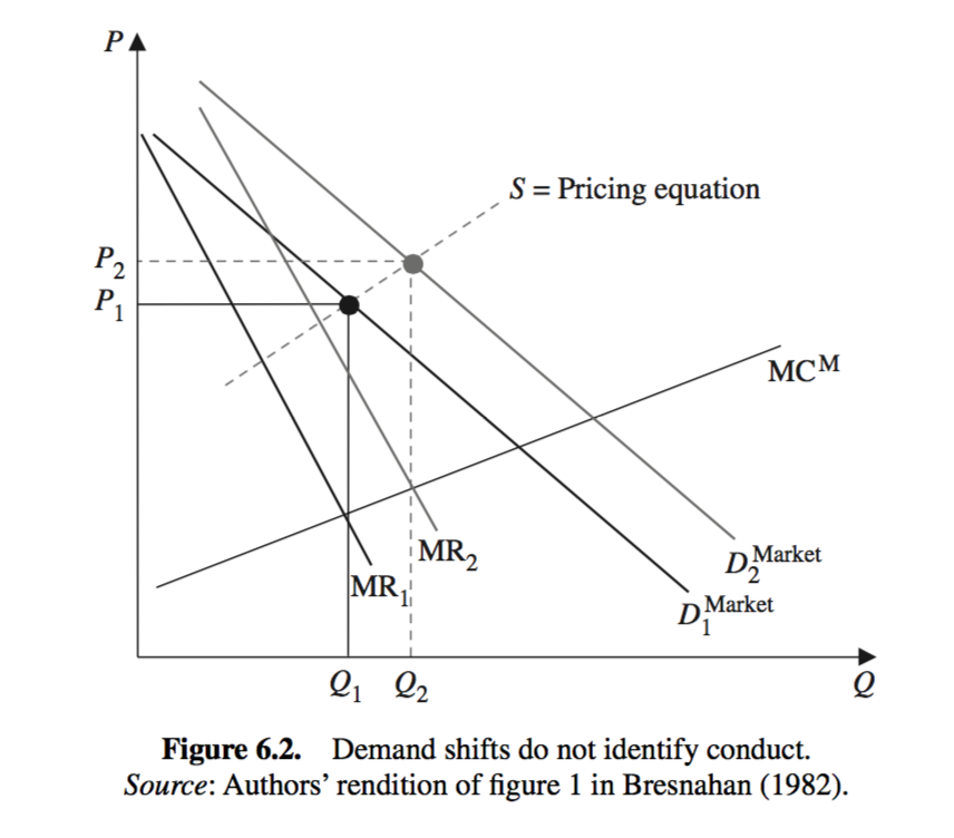
Figure 5.1: Figure 6.2 of Davis (2006)
5.2.8 Identification of the Conduct Parameter: When Cost Data is Available
- If there is reliable cost data, we can directly identify the marginal cost function: \[\begin{equation} MC(q_f) = \beta_0 + \beta_1 q_f + \beta_2 W + u^S, \end{equation}\] and so \(\beta_1\).
- Then, in a combination with the identification of inverse demand function and pricing equation, \(\lambda\) is identified as: \[\begin{equation} \lambda = \alpha_1 \left(\frac{\beta_1}{N} - \gamma\right). \end{equation}\]
5.2.9 Identification of the Conduct Parameter: When Cost Data is Not Available
- Remember the first-order condition: \[\begin{equation} \lambda Q P^{D\prime}(Q) + P^S(Q) = MC(q_f), \end{equation}\] where we can identify \(P^D(Q)\) and \(P^S(Q)\) if we have demand and cost shifters.
- It is clear from this expression that we need a variation in \(P^{D\prime}(Q)\) with a fixed \(Q\) to identify \(\lambda\), i.e., something that rotates the inverse demand function.
- Intuition: If demand becomes more elastic, prices will decrease and quantity will increase in a market with a high degree of market power.
5.2.10 Identification of the Conduct Parameter: Demand Rotater is Available
Let’s formalize the idea.
To identify the conduct parameter, we needed a demand rotater: \[\begin{equation} P^D(Q) = \frac{\alpha_0}{\alpha_1} + \frac{1}{\alpha_1}Q + \frac{\alpha_2}{\alpha_1} X + \frac{\alpha_3}{\alpha_1} Q \underbrace{Z}_{\text{demand rotater}} + \frac{1}{\alpha_1}u^D. \end{equation}\]
Inserting this into the first-order condition yields: \[\begin{equation} \frac{\lambda}{\alpha} Q_t (1 + \alpha Z_t)+ P^S(Q) = \beta_0 + \frac{\beta_1}{N} Q + \beta_2 W + u^s, \end{equation}\]
This determines the pricing equation: \[\begin{equation} \begin{split} P^S(Q) &= \beta_0 - \frac{\lambda}{\alpha_1} Q(1 + \alpha_3 Z_t) + \frac{\beta_1}{N} Q_t + \beta_2 W + u^S\\ &\equiv \beta_0 + \gamma_1 Q + \gamma_2 Z Q + \beta_2 W + u^S, \end{split} \end{equation}\] where: \[\begin{equation} \gamma_1 \equiv \frac{\beta_1}{N} - \frac{\lambda}{\alpha_1}, \gamma_2 \equiv - \frac{\lambda \alpha_3}{\alpha_1}. \end{equation}\] ### Identification of the Conduct Parameters: Demand Rotater is Available
If we have cost shifters \(W\), it can be used as instruments for \(Q\) in the inverse demand function to identify the demand parameters \((\alpha_0, \alpha_1, \alpha_2, \alpha_3)\).
If we have demand shifters \(X\), it can be used as instruments for \(Q\) in the pricing equation to identify the supply parameters \((\beta_0, \gamma_1, \gamma_2, \beta_2)\).
Now we can identify the reduced-form parameters \(\alpha_1, \alpha_3\) and \(\gamma_2\).
Then, we can not identify the conduct parameter: \[\begin{equation} \lambda = - \frac{\gamma_2 \alpha_1}{\alpha_3}. \end{equation}\]
5.2.11 Identification of Conduct in Differentiated Product Market
Consider the identification of conduct when there are two differentiated substitutable products and companies compete in price (Nevo, 1998).
Are the prices determined independently or jointly?
The general first-order condition is: \[\begin{equation} \begin{split} &(p_1 - c_1) \frac{\partial Q_1(p)}{\partial p_1} + Q_1^S(p) + \Delta_{12}(p_2 - c_2) \frac{\partial Q_2 (p)}{\partial p_1} = 0\\ &\Delta_{21}(p_1 - c_1)\frac{\partial Q_1(p)}{\partial p_2} + Q_2^S(p) + (p_2 - c_2) \frac{\partial Q_2 (p)}{\partial p_2} = 0, \end{split} \end{equation}\] where
\(\Delta_{12} = \Delta_{21} = 0\) if prices are determined independently.
\(\Delta_{12} = \Delta_{21} = 1\) if price are determined jointly.
Under what conditions can we identify \(\Delta_{12}\) and \(\Delta_{21}\)?
We will have to rotate \(\frac{\partial Q_1(p)}{\partial p_2}\) and \(\frac{\partial Q_2 (p)}{\partial p_1}\) while keeping the other variables at the same values.
Miller & Weinberg (2017) infers \(\Delta\) after the MillerCoors, a joint venture of SABMiller PLC and Molson Coors Brewing, is formed.
- The unobserved year-specific and region-specific cost shocks are identified from the outsiders and the unobserved product-specific cost shocks are assumed to be the same before and after the merger.
5.3 Merger Simulation
5.3.1 Unilateral and Coordinated Effects of a Horizontal Merger
- There are two effects associated with a merge episode:
- Unilateral effect:
- The new merged firm usually have a unilateral incentive to raise prices above their pre-merger level.
- This unilateral effect may lead to the other firms to have an unilateral incentive to raise price, and the reaction continues to reach the new equilibrium.
- The latter chain reaction is sometimes called the multi-lateral effect.
- In economic theory, it is the price change when the same mode of competition (say, the Bertrand-Nash equilibrium) is played.
- \(\Delta\) is either 0 or 1: firms internalize the profits from owned product but do not internalize the other products.
- Coordinated effect:
- After the merger, the mode of competition may change.
- For example, the tacit collusion becomes easier and it can happen.
- This effect, caused by the change in the mode of competition, is called the coordinated effect of a merger.
- In this case, the conduct parameters \(\Delta\) may take positive values for products owned by the rival firms.
5.3.2 Merger Simulation
- In merger simulation, we compute the equilibrium under different ownership structure.
- This amounts to run a counterfactual simulation hypothetically changing the conduct parameter \(\Delta\).
- The idea stems back to Farrell & Shapiro (1990), Werden & Frobe (1993), Hausman et al. (1994).
- Before running the simulation, you have to be very careful about the model assumptions:
- In music industry, firms compete not in price but in advertisement.
- If technological diffusion is important, firms may set dynamic pricing.
- This is the first counterfactual analysis we study in this lecture.
- The results are valid only if the modeling assumptions are correct.
5.3.3 Quantifying the Unilateral Effect
- See Nevo (2000) and Nevo (2001).
- There are \(J\) products, \(\mathcal{J} = \{1, \cdots, J\}\).
- We can have multiple markets but we suppress the market index.
- Firm \(f\) produces a set of products which we denote \(\mathcal{J}_f \subset \mathcal{J}\).
- Let \(mc_j\) be the constant marginal cost of producing good \(j\).
- Thus assuming a separable cost function.
- We can relax this assumption for the estimation.
- However, once you admit that the costs can be non-separable, you will start to wonder what happens to the cost function if two firms merged and started to produce the two products that were previously produced by separate firms.
- Let \(D_j(p)\) be the demand for product \(j\) when the price vector is \(p\).
- The problem for firm \(f\) given the price of other firms \(p_{-f}\) is: \[\begin{equation} \max_{p_f} \sum_{j \in \mathcal{J}_f} \Pi_j(p_f, p_{-f}) = \sum_{j \in \mathcal{J}_f} (p_j - mc_j) D_j(p_f, p_{-f}), \end{equation}\] where \(p_f = \{p_j\}_{j \in \mathcal{J}_f}\), \(p_{-f} = \{p_j\}_{j \in \mathcal{J} \setminus \mathcal{J}_f}\).
5.3.4 Pre-Merger Equilibrium
- The first-order condition for firm \(f\) is: \[\begin{equation} D_k(p) + \sum_{j \in \mathcal{J}_f} (p_j - mc_j) \frac{\partial D_j(p)}{\partial p_k} = 0, \forall k \in \mathcal{J}_f. \end{equation}\]
- Let \(\Delta_{jk}^{pre}\) takes 1 if same firm produces \(j\) and \(k\) and 0 otherwise before the merger.
- The first-order condition can be written as: \[\begin{equation} D_k(p) + \sum_{j \in \mathcal{J}} \Delta_{jk}^{pre}(p_j - mc_j) \frac{\partial D_j(p)}{\partial p_k} = 0, \forall k \in \mathcal{J}_f. \end{equation}\]
- In terms of the product share: \[\begin{equation} s_k(p) + \sum_{j \in \mathcal{J}} \Delta_{jk}^{pre}(p_j - mc_j) \frac{\partial s_j(p)}{\partial p_k} = 0, \forall k \in \mathcal{J}_f. \end{equation}\]
- Let \(\Delta^{pre}\) be a \(J \times J\) matrix whose \((j, k)\)-element is \(\Delta_{jk}\).
- At the end of the day, performing a merger simulation is to recompute the equilibrium with different ownership structure encoded in \(\Delta\).
5.3.5 Post-Merger Equilibrium
- Let \(\Omega^{pre}(p)\) is a matrix whose \((j, k)\)-element is:
\[\begin{equation} - \frac{\partial s_{j}(p)}{\partial p_k} \Delta_{jk}^{pre}. \end{equation}\]
Then, by the first-order condition, the marginal cost should be: \[\begin{equation} mc = p - \Omega^{pre}(p)^{-1} s(p). \end{equation}\]
If the ownership structure \(\Delta^{pre}\) is changed to \(\Delta^{post}\), and \(\Omega^{pre}\) changed to \(\Omega^{post}\), the post-merger price is determined by solving the non-linear equation: \[\begin{equation} p^{post} = mc + \Omega^{post}(p^{post})^{-1}s(p^{post}). \end{equation}\]
The post-merger share is given by: \[\begin{equation} s^{post} = s(p^{post}). \end{equation}\]
5.3.6 Consumer Surplus
- Suppose that the demand function is based on the mixed-logit model such that the indirect utility is: \[\begin{equation} u_{ijt} = x_{jt} \beta_i + \alpha_i p_{jt} + \xi_{j} + \xi_t + \Delta \xi_{jt} + \epsilon_{ijt}, \end{equation}\] with \(\epsilon_{ijt}\) is drawn from i.i.d. Type-I extreme value distribution and the consumer-level heterogeneity:
\[\begin{equation} \begin{pmatrix} \alpha_i \\ \beta_i \end{pmatrix} = \begin{pmatrix} \alpha\\ \beta \end{pmatrix} + \Pi z_i + \Sigma \nu_i, \nu_i \sim N(0, I_{K + 1}). \end{equation}\]
- Then, the compensated variation due to the price change for consumer \(i\) is: \[\begin{equation} CV_{it} = \frac{\ln (\sum_{j = 0}^J \exp(V_{ijt}^{post}) ) - \ln (\sum_{j = 0}^J \exp(V_{ijt}^{pre})) }{\alpha_i}, \end{equation}\] where \(V_{ijt}^{post}\) and \(V_{ijt}^{pre}\) are indirect utility for consumer \(i\) to purchase good \(j\) at the prices after and before the merger.
- This formula holds only if the price enters linearly in the indirect utility (no income effect).
- For general case, see Small & Rosen (1981) and D. Mcfadden et al. (1995).
5.3.7 Quantifying the Coordinated Effect
- The repeated-game theory suggests that a collusion is sustainable if and only if it it incentive compatible: the collusion profit is no less than the deviation profit for each member of the collusion.
- The theory provides a check list that affects the incentive compatibility such as the market share, cost asymmetry, and demand dynamics.
- But it is often hard to judge the coordinated effects from these qualitative information, because mergers simultaneously change many factors and the factors may encourage or hinder collusion.
- Miller & Weinberg (2017) retrospectively studies the coordinated effect of a merger.
- Is prospective analysis of coordinated effects possible as well as the analysis of unilateral effects?
- If we can identify the demand and cost functions, we can calculate the collusion profits and deviation profits.
- If we specify the collusion strategy, we can write down the incentive compatibility.
- We can check how the incentive compatibility change when a hypothetical merger happens.
- The problem is the identification of conduct: to identify the cost function, we need to know the conduct.
- Thus, the stated strategy will work only if we have a data during which we are sure that there was no collusion, or there was a particular type of collusion.
- Igami & Sugaya (2018) use the detailed information of vitamin C cartel case and apply this approach.