Chapter 11 Assignment 1: Basic Programming in R

Report the following results in html format using R markdown. In other words, replicate this document. You write functions in a separate R file and put in R folder in the project folder. Build the project as a package and load it from the R markdown file. The execution code sholuld be written in R markdown file.

You submit:

R file containing functions.
R markdown file containing your answers and executing codes.
HTML(or PDF) report generated from the R markdown.

11.1 Simulate data

Consider to simulate data from the following model and estimate the parameters from the simulated data.

\[ y_{ij} = 1\{j = \text{argmax}_{k = 1, 2} \beta x_k + \epsilon_{ik} \}, \] where \(\epsilon_{ik}\) follows i.i.d. type-I extreme value distribution, \(\beta = 0.2\), \(x_1 = 0\) and \(x_2 = 1\).

To simulate data, first make a data frame as follows:

df

## # A tibble: 2,000 × 3
##        i     k     x
##    <int> <int> <dbl>
##  1     1     1     0
##  2     1     2     1
##  3     2     1     0
##  4     2     2     1
##  5     3     1     0
##  6     3     2     1
##  7     4     1     0
##  8     4     2     1
##  9     5     1     0
## 10     5     2     1
## # ℹ 1,990 more rows

Second, draw type-I extreme value random variables. Set the seed at 1. You can use evd package to draw the variables. You should get exactly the same realization if the seed is correctly set.

set.seed(1)

df

## # A tibble: 2,000 × 4
##        i     k     x       e
##    <int> <int> <dbl>   <dbl>
##  1     1     1     0  0.281 
##  2     1     2     1 -0.167 
##  3     2     1     0  1.93  
##  4     2     2     1  1.97  
##  5     3     1     0  0.830 
##  6     3     2     1 -1.06  
##  7     4     1     0 -0.207 
##  8     4     2     1  0.617 
##  9     5     1     0  0.0444
## 10     5     2     1  1.92  
## # ℹ 1,990 more rows

Third, compute the latent value of each option to obtain the following data frame:

beta <- 0.2

df

## # A tibble: 2,000 × 5
##        i     k     x       e  latent
##    <int> <int> <dbl>   <dbl>   <dbl>
##  1     1     1     0  0.281   0.281 
##  2     1     2     1 -0.167   0.0331
##  3     2     1     0  1.93    1.93  
##  4     2     2     1  1.97    2.17  
##  5     3     1     0  0.830   0.830 
##  6     3     2     1 -1.06   -0.863 
##  7     4     1     0 -0.207  -0.207 
##  8     4     2     1  0.617   0.817 
##  9     5     1     0  0.0444  0.0444
## 10     5     2     1  1.92    2.12  
## # ℹ 1,990 more rows

Finally, compute \(y\) by comparing the latent values of \(k = 1, 2\) for each \(i\) to obtain the following result:

df

## # A tibble: 2,000 × 6
##        i     k     x       e  latent     y
##    <int> <int> <dbl>   <dbl>   <dbl> <dbl>
##  1     1     1     0  0.281   0.281      1
##  2     1     2     1 -0.167   0.0331     0
##  3     2     1     0  1.93    1.93       0
##  4     2     2     1  1.97    2.17       1
##  5     3     1     0  0.830   0.830      1
##  6     3     2     1 -1.06   -0.863      0
##  7     4     1     0 -0.207  -0.207      0
##  8     4     2     1  0.617   0.817      1
##  9     5     1     0  0.0444  0.0444     0
## 10     5     2     1  1.92    2.12       1
## # ℹ 1,990 more rows

11.2 Estimate the parameter

Now you generated simulated data. Suppose you observe \(x_k\) and \(y_{ik}\) for each \(i\) and \(k\) and estimate \(\beta\) by a maximum likelihood estimator. The likelihood for \(i\) to choose \(k\) (\(y_{ik} = 1\)) can be shown to be: \[ p_{ik}(\beta) = \frac{\exp(\beta x_k)}{\exp(\beta x_1) + \exp(\beta x_2)}. \]

Then, the likelihood of observing \(\{y_{ik}\}_{i, k}\) is: \[ L(\beta) = \prod_{i = 1}^{1000} p_{i1}(\beta)^{y_{i1}} [1 - p_{i1}(\beta)]^{1 - y_{i1}}, \] and the log likelihood is: \[ l(\beta) = \sum_{i = 1}^{1000}\{y_{i1}\log p_{i1}(\beta) + (1 - y_{i1})\log [1 - p_{i1}(\beta)\}. \]

Write a function to compute the likelihood for a given \(\beta\) and data and name the function compute_loglikelihood_a1(b, df).

compute_loglikelihood_a1(
    b = 1,
    df = df
  )

## [1] -0.7542617

Compute the value of log likelihood for \(\beta = 0, 0.1, \cdots, 1\) and plot the result using ggplot2 packages. You can use latex2exp package to use LaTeX math symbol in the label:

b_seq <- seq(0, 1, 0.1)
output <- 
  foreach (
    b = b_seq,
    .combine = "rbind"
    ) %do% {
      l <- 
        compute_loglikelihood_a1(
          b, 
          df
          )
      return(l)
}
output <- 
  data.frame(
    x = b_seq, 
    y = output
    )
output %>%
  ggplot(
    aes(
      x = x, 
      y = y
      )
    ) +
  geom_point() + 
  xlab(TeX("$\\beta$")) + 
  ylab("Loglikelihood") +
  theme_classic()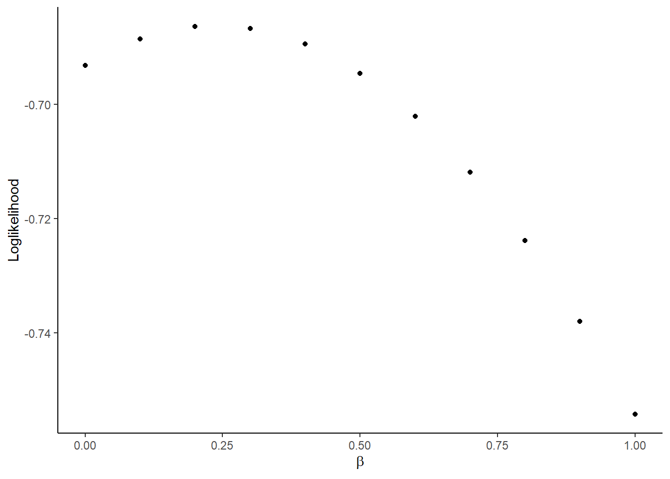

Find and report \(\beta\) that maximizes the log likelihood for the simulated data. You can use optim function to achieve this. You will use Brent method and set the lower bound at -1 and upper bound at 1 for the parameter search.

## $par
## [1] 0.2371046
## 
## $value
## [1] -0.6861689
## 
## $counts
## function gradient 
##       NA       NA 
## 
## $convergence
## [1] 0
## 
## $message
## NULL