Chapter 18 Assignment 8: Dynamic Game

18.1 Simulate data

Suppose that there are \(m = 1, \cdots, M\) markets and in each market there are \(i = 1, \cdots, N\) firms and each firm makes decisions for \(t = 1, \cdots, \infty\). In the following, I suppress the index of market, \(m\). We solve the model under the infinite-horizon assumption, but generate data only for \(t = 1, \cdots, T\). There are \(L = 5\) state \(\{1, 2, 3, 4, 5\}\) states for each firm. Each firm can choose \(K + 1 = 2\) actions \(\{0, 1\}\). Thus, \(m_a := (K + 1)^N\) and \(m_s = L^N\). Let \(a_i\) and \(s_i\) be firm \(i\)’s action and state and \(a\) and \(s\) are vectors of individual actions and states.

The mean period payoff to firm \(i\) is: \[ \pi_i(a, s) := \tilde{\pi}(a_i, s_i, \overline{s}) := \alpha \ln s_i - \eta \ln s_i \sum_{j \neq i} \ln s_j - \beta a_i, \] where \(\alpha, \beta, \eta> 0\), and \(\alpha > \eta\). The term \(\eta\) means that the returns to investment decreases as rival’s average state profile improves. The period payoff is: \[ \tilde{\pi}(a_i, s_i, \overline{s})+ \epsilon_i(a_i), \] and \(\epsilon_i(a_i)\) is an i.i.d. type-I extreme random variable that is independent of all the other variables.

At the beginning of each period, the state \(s\) is realized and publicly observed. Then choice-specific shocks \(\epsilon_i(a_i), a_i = 0, 1\) are realized and privately observed by firm \(i = 1, \cdots, N\). Then each firm simultaneously chooses her action. Then, the game moves to next period.

State transition is independent across firms conditional on individual state and action.

Suppose that \(s_i > 1\) and \(s_i < L\). If \(a_i = 0\), the state stays at the same state with probability \(1 - \kappa\) and moves down by 1 with probability \(\kappa\). If \(a = 1\), the state moves up by 1 with probability \(\gamma\), moves down by 1 with probability \(\kappa\), and stays at the same with probability \(1 - \kappa - \gamma\).

Suppose that \(s_i = 1\). If \(a_i = 0\), the state stays at the same state with probability 1. If \(a_i = 1\), the state moves up by 1 with probability \(\gamma\) and stays at the same with probability \(1 - \gamma\).

Suppose that \(s_i = L\). If \(a_i = 0\), the state stays at the same state with probability \(1 - \kappa\) and moves down by 1 with probability \(\kappa\). If \(a = 1\), the state moves down by 1 with probability \(\kappa\), and stays at the same with probability \(1 - \kappa\).

The mean period profit is summarized in \(\Pi\) as:

\[ \Pi := \begin{pmatrix} \pi(1, 1)\\ \vdots\\ \pi(m_a, 1)\\ \vdots \\ \pi(1, m_s)\\ \vdots\\ \pi(m_a, m_s)\\ \end{pmatrix} \]

The transition law is summarized in \(G\) as:

\[ g(a, s, s') := \mathbb{P}\{s_{t + 1} = s'|s_t = s, a_t = a\}, \]

\[ G := \begin{pmatrix} g(1, 1, 1) & \cdots & g(1, 1, m_s)\\ \vdots & & \vdots \\ g(m_a, 1, 1) & \cdots & g(m_a, 1, m_s)\\ & \vdots & \\ g(1, m_s, 1) & \cdots & g(1, m_s, m_s)\\ \vdots & & \vdots \\ g(m_a, m_s, 1) & \cdots & g(m_a, m_s, m_s)\\ \end{pmatrix}. \] The discount factor is denoted by \(\delta\). We simulate data for \(M\) markets with \(N\) firms for \(T\) periods.

1. Set constants and parameters as follows:

# set seed
set.seed(1)
# set constants 
L <- 5
K <- 1
T <- 100
N <- 3
M <- 1000
lambda <- 1e-10
# set parameters
alpha <- 1
eta <- 0.3
beta <- 2
kappa <- 0.1
gamma <- 0.6
delta <- 0.95

2. Write a function compute_action_state_space(K, L, N) that returns a data frame for action and state space. Returned objects are list of data frame A and S. In A, column k is the index of an action profile, i is the index of a firm, and a is the action of the firm. In S, column l is the index of an state profile, i is the index of a firm, and s is the state of the firm.

output <- 
  compute_action_state_space(
    L = L,
    K = K, 
    N = N
    )
A <- output$A
head(A)

## # A tibble: 6 × 3
##       k     i     a
##   <int> <int> <int>
## 1     1     1     0
## 2     1     2     0
## 3     1     3     0
## 4     2     1     1
## 5     2     2     0
## 6     2     3     0

tail(A)

## # A tibble: 6 × 3
##       k     i     a
##   <int> <int> <int>
## 1     7     1     0
## 2     7     2     1
## 3     7     3     1
## 4     8     1     1
## 5     8     2     1
## 6     8     3     1

S <- output$S
head(S)

## # A tibble: 6 × 3
##       l     i     s
##   <int> <int> <int>
## 1     1     1     1
## 2     1     2     1
## 3     1     3     1
## 4     2     1     2
## 5     2     2     1
## 6     2     3     1

tail(S)

## # A tibble: 6 × 3
##       l     i     s
##   <int> <int> <int>
## 1   124     1     4
## 2   124     2     5
## 3   124     3     5
## 4   125     1     5
## 5   125     2     5
## 6   125     3     5

# dimension
m_a <- max(A$k); 
m_a

## [1] 8

m_s <- max(S$l); 
m_s

## [1] 125

3. Write function compute_PI_game(alpha, beta, eta, A, S) that returns a list of \(\Pi_i\).

PI <- 
  compute_PI_game(
    alpha = alpha, 
    beta = beta, 
    eta = eta, 
    A = A,
    S = S
    )
head(PI[[N]])

##      [,1]
## [1,]    0
## [2,]    0
## [3,]    0
## [4,]    0
## [5,]   -2
## [6,]   -2

dim(PI[[N]])[1] == m_s * m_a

## [1] TRUE

4. Write function compute_G_game(g, A, S) that converts an individual transition probability matrix into a joint transition probability matrix \(G\).

G_marginal <- 
  compute_G(
    kappa = kappa,
    gamma = gamma, 
    L = L, 
    K = K
    )
G <- 
  compute_G_game(
    G_marginal = G_marginal, 
    A = A, 
    S = S
    )
head(G)

##         1    2 3 4 5    6    7 8 9 10 11 12 13 14 15 16 17 18 19 20 21 22 23 24 25
## [1,] 1.00 0.00 0 0 0 0.00 0.00 0 0  0  0  0  0  0  0  0  0  0  0  0  0  0  0  0  0
## [2,] 0.40 0.60 0 0 0 0.00 0.00 0 0  0  0  0  0  0  0  0  0  0  0  0  0  0  0  0  0
## [3,] 0.40 0.00 0 0 0 0.60 0.00 0 0  0  0  0  0  0  0  0  0  0  0  0  0  0  0  0  0
## [4,] 0.16 0.24 0 0 0 0.24 0.36 0 0  0  0  0  0  0  0  0  0  0  0  0  0  0  0  0  0
## [5,] 0.40 0.00 0 0 0 0.00 0.00 0 0  0  0  0  0  0  0  0  0  0  0  0  0  0  0  0  0
## [6,] 0.16 0.24 0 0 0 0.00 0.00 0 0  0  0  0  0  0  0  0  0  0  0  0  0  0  0  0  0
##        26   27 28 29 30 31 32 33 34 35 36 37 38 39 40 41 42 43 44 45 46 47 48 49 50
## [1,] 0.00 0.00  0  0  0  0  0  0  0  0  0  0  0  0  0  0  0  0  0  0  0  0  0  0  0
## [2,] 0.00 0.00  0  0  0  0  0  0  0  0  0  0  0  0  0  0  0  0  0  0  0  0  0  0  0
## [3,] 0.00 0.00  0  0  0  0  0  0  0  0  0  0  0  0  0  0  0  0  0  0  0  0  0  0  0
## [4,] 0.00 0.00  0  0  0  0  0  0  0  0  0  0  0  0  0  0  0  0  0  0  0  0  0  0  0
## [5,] 0.60 0.00  0  0  0  0  0  0  0  0  0  0  0  0  0  0  0  0  0  0  0  0  0  0  0
## [6,] 0.24 0.36  0  0  0  0  0  0  0  0  0  0  0  0  0  0  0  0  0  0  0  0  0  0  0
##      51 52 53 54 55 56 57 58 59 60 61 62 63 64 65 66 67 68 69 70 71 72 73 74 75 76 77
## [1,]  0  0  0  0  0  0  0  0  0  0  0  0  0  0  0  0  0  0  0  0  0  0  0  0  0  0  0
## [2,]  0  0  0  0  0  0  0  0  0  0  0  0  0  0  0  0  0  0  0  0  0  0  0  0  0  0  0
## [3,]  0  0  0  0  0  0  0  0  0  0  0  0  0  0  0  0  0  0  0  0  0  0  0  0  0  0  0
## [4,]  0  0  0  0  0  0  0  0  0  0  0  0  0  0  0  0  0  0  0  0  0  0  0  0  0  0  0
## [5,]  0  0  0  0  0  0  0  0  0  0  0  0  0  0  0  0  0  0  0  0  0  0  0  0  0  0  0
## [6,]  0  0  0  0  0  0  0  0  0  0  0  0  0  0  0  0  0  0  0  0  0  0  0  0  0  0  0
##      78 79 80 81 82 83 84 85 86 87 88 89 90 91 92 93 94 95 96 97 98 99 100 101 102
## [1,]  0  0  0  0  0  0  0  0  0  0  0  0  0  0  0  0  0  0  0  0  0  0   0   0   0
## [2,]  0  0  0  0  0  0  0  0  0  0  0  0  0  0  0  0  0  0  0  0  0  0   0   0   0
## [3,]  0  0  0  0  0  0  0  0  0  0  0  0  0  0  0  0  0  0  0  0  0  0   0   0   0
## [4,]  0  0  0  0  0  0  0  0  0  0  0  0  0  0  0  0  0  0  0  0  0  0   0   0   0
## [5,]  0  0  0  0  0  0  0  0  0  0  0  0  0  0  0  0  0  0  0  0  0  0   0   0   0
## [6,]  0  0  0  0  0  0  0  0  0  0  0  0  0  0  0  0  0  0  0  0  0  0   0   0   0
##      103 104 105 106 107 108 109 110 111 112 113 114 115 116 117 118 119 120 121 122
## [1,]   0   0   0   0   0   0   0   0   0   0   0   0   0   0   0   0   0   0   0   0
## [2,]   0   0   0   0   0   0   0   0   0   0   0   0   0   0   0   0   0   0   0   0
## [3,]   0   0   0   0   0   0   0   0   0   0   0   0   0   0   0   0   0   0   0   0
## [4,]   0   0   0   0   0   0   0   0   0   0   0   0   0   0   0   0   0   0   0   0
## [5,]   0   0   0   0   0   0   0   0   0   0   0   0   0   0   0   0   0   0   0   0
## [6,]   0   0   0   0   0   0   0   0   0   0   0   0   0   0   0   0   0   0   0   0
##      123 124 125
## [1,]   0   0   0
## [2,]   0   0   0
## [3,]   0   0   0
## [4,]   0   0   0
## [5,]   0   0   0
## [6,]   0   0   0

dim(G)[1] == m_s * m_a

## [1] TRUE

dim(G)[2] == m_s

## [1] TRUE

The ex-ante-value function for a firm is written as a function of a conditional choice probability as follows: \[ \varphi_i^{(\theta_1, \theta_2)}(p) := [I - \delta \Sigma(p) G]^{-1}[\Sigma(p)\Pi_i + D_i(p)], \] where \(\theta_1 = (\alpha, \beta, \eta)\) and \(\theta_2 = (\kappa, \gamma)\), \(p_i(a_i|s)\) is the probability that firm \(i\) choose action \(a_i\) when the state profile is \(s\), and: \[ p(a|s) = \prod_{i = 1}^N p_i(a_i|s), \]

\[ p(s) = \begin{pmatrix} p(1|s) \\ \vdots \\ p(m_a|s) \end{pmatrix}, \]

\[ p = \begin{pmatrix} p(1)\\ \vdots\\ p(m_s) \end{pmatrix}, \]

\[ \Sigma(p) = \begin{pmatrix} p(1)' & & \\ & \ddots & \\ & & p(L)' \end{pmatrix} \]

and:

\[ D_i(p) = \begin{pmatrix} \sum_{k = 0}^K \mathbb{E}\{\epsilon_i^k|a_i = k, 1\}p_i(a_i = k|1)\\ \vdots\\ \sum_{k = 0}^K \mathbb{E}\{\epsilon_i^k|a_i = k, m_s\}p_i(a_i = k|m_s) \end{pmatrix}. \]

5. Write a function initialize_p_marginal(A, S) that defines an initial marginal condition choice probability. In the output p_marginal, p is the probability for firm i to take action a conditional on the state profile being l. Next, write a function compute_p_joint(p_marginal, A, S) that computes a corresponding joint conditional choice probability from a marginal conditional choice probability. In the output p_joint, p is the joint probability that firms take action profile k condition on the state profile being l. Finally, write a function compute_p_marginal(p_joint, A, S) that compute a corresponding marginal conditional choice probability from a joint conditional choice probability.

# define a conditional choice probability for each firm
p_marginal <- 
  initialize_p_marginal(
    A = A,
    S = S
    )
p_marginal

## # A tibble: 750 × 4
##        i     l     a     p
##    <int> <int> <int> <dbl>
##  1     1     1     0   0.5
##  2     1     1     1   0.5
##  3     1     2     0   0.5
##  4     1     2     1   0.5
##  5     1     3     0   0.5
##  6     1     3     1   0.5
##  7     1     4     0   0.5
##  8     1     4     1   0.5
##  9     1     5     0   0.5
## 10     1     5     1   0.5
## # ℹ 740 more rows

dim(p_marginal)[1] == N * m_s * (K + 1)

## [1] TRUE

# compute joint conditional choice probability from marginal probability
p_joint <- 
  compute_p_joint(
    p_marginal = p_marginal, 
    A = A, 
    S = S
    )
p_joint

## # A tibble: 1,000 × 3
##        l     k     p
##    <int> <int> <dbl>
##  1     1     1 0.125
##  2     1     2 0.125
##  3     1     3 0.125
##  4     1     4 0.125
##  5     1     5 0.125
##  6     1     6 0.125
##  7     1     7 0.125
##  8     1     8 0.125
##  9     2     1 0.125
## 10     2     2 0.125
## # ℹ 990 more rows

dim(p_joint)[1] == m_s * m_a

## [1] TRUE

# compute marginal conditional choice probability from joint probability
p_marginal_2 <- 
  compute_p_marginal(
    p_joint = p_joint, 
    A = A,
    S = S
    )
max(abs(p_marginal - p_marginal_2))

## [1] 0

6. Write a function compute_sigma(p_marginal, A, S) that computes \(\Sigma(p)\) given a joint conditional choice probability. Then, write a function compute_D(p_marginal) that returns a list of \(D_i(p)\).

# compute Sigma for ex-ante value function calculation
sigma <- 
  compute_sigma(
    p_marginal = p_marginal,
    A = A,
    S = S
    )
head(sigma)

## 6 x 1000 sparse Matrix of class "dgCMatrix"
##                                                                                   
## [1,] 0.125 0.125 0.125 0.125 0.125 0.125 0.125 0.125 .     .     .     .     .    
## [2,] .     .     .     .     .     .     .     .     0.125 0.125 0.125 0.125 0.125
## [3,] .     .     .     .     .     .     .     .     .     .     .     .     .    
## [4,] .     .     .     .     .     .     .     .     .     .     .     .     .    
## [5,] .     .     .     .     .     .     .     .     .     .     .     .     .    
## [6,] .     .     .     .     .     .     .     .     .     .     .     .     .    
##                                                                                   
## [1,] .     .     .     .     .     .     .     .     .     .     .     .     .    
## [2,] 0.125 0.125 0.125 .     .     .     .     .     .     .     .     .     .    
## [3,] .     .     .     0.125 0.125 0.125 0.125 0.125 0.125 0.125 0.125 .     .    
## [4,] .     .     .     .     .     .     .     .     .     .     .     0.125 0.125
## [5,] .     .     .     .     .     .     .     .     .     .     .     .     .    
## [6,] .     .     .     .     .     .     .     .     .     .     .     .     .    
##                                                                              
## [1,] .     .     .     .     .     .     .     .     .     .     .     ......
## [2,] .     .     .     .     .     .     .     .     .     .     .     ......
## [3,] .     .     .     .     .     .     .     .     .     .     .     ......
## [4,] 0.125 0.125 0.125 0.125 0.125 0.125 .     .     .     .     .     ......
## [5,] .     .     .     .     .     .     0.125 0.125 0.125 0.125 0.125 ......
## [6,] .     .     .     .     .     .     .     .     .     .     .     ......
## 
##  .....suppressing 963 columns in show(); maybe adjust 'options(max.print= *, width = *)'
##  ..............................

dim(sigma)[1] == m_s

## [1] TRUE

dim(sigma)[2] == m_s * m_a

## [1] TRUE

# compute D for ex-ante value function calculation
D <- compute_D(p_marginal)
head(D[[N]])

##          [,1]
## [1,] 1.270363
## [2,] 1.270363
## [3,] 1.270363
## [4,] 1.270363
## [5,] 1.270363
## [6,] 1.270363

dim(D[[N]])[1] == m_s

## [1] TRUE

7. Write a function compute_exante_value_game(p_marginal, A, S, PI, G, delta) that returns a list of matrices whose \(i\)-th element represents the ex-ante value function given a conditional choice probability for firm \(i\).

# compute ex-ante value funciton for each firm
V <- 
  compute_exante_value_game(
    p_marginal = p_marginal,
    A = A,
    S = S,
    PI = PI,
    G = G,
    delta = delta
    )
head(V[[N]])

## 6 x 1 Matrix of class "dgeMatrix"
##         [,1]
## l1 10.786330
## l2 10.175982
## l3  9.606812
## l4  9.255459
## l5  9.115332
## l6 10.175982

dim(V[[N]])[1] == m_s

## [1] TRUE

The optimal conditional choice probability is written as a function of an ex-ante value function and a conditional choice probability of others as follows: \[ \Lambda_i^{(\theta_1, \theta_2)}(V_i, p_{-i})(a_i, s) := \frac{\exp\{\sum_{a_{-i}}p_{-i}(a_{-i}|s)[\pi_i(a_i, a_{-i}, s) + \delta \sum_{s'}V_i(s')g(a_i, a_{-i}, s, s')]\}}{\sum_{a_i'}\exp\{\sum_{a_{-i}}p_{-i}(a_{-i}|s)[\pi_i(a_i', a_{-i}, s) + \delta \sum_{s'}V_i(s')g(a_i', a_{-i}, s, s')]\}}, \] where \(V\) is an ex-ante value function.

8. Write a function compute_profile_value_game(V, PI, G, delta, S, A) that returns a data frame that contains information on value function at a state and action profile for each firm. In the output value, i is the index of a firm, l is the index of a state profile, k is the index of an action profile, and value is the value for the firm at the state and action profile.

# compute state-action-profile value function
value <- 
  compute_profile_value_game(
    V = V, 
    PI = PI,
    G = G, 
    delta = delta, 
    S = S, 
    A = A
    )
value

## # A tibble: 3,000 × 4
##        i     l     k value
##    <int> <int> <int> <dbl>
##  1     1     1     1 10.2 
##  2     1     1     2  9.63
##  3     1     1     3  9.90
##  4     1     1     4  9.13
##  5     1     1     5  9.90
##  6     1     1     6  9.13
##  7     1     1     7  9.55
##  8     1     1     8  8.64
##  9     1     2     1 13.0 
## 10     1     2     2 12.1 
## # ℹ 2,990 more rows

dim(value)[1] == N * m_s * m_a

## [1] TRUE

9. Write a function compute_choice_value_game(p_marginal, V, PI, G, delta, A, S) that computes a data frame that contains information on a choice-specific value function given an ex-ante value function and a conditional choice probability of others.

# compute choice-specific value function
value <- 
  compute_choice_value_game(
    p_marginal = p_marginal,
    V = V,
    PI = PI,
    G = G, 
    delta = delta, 
    A = A, 
    S = S
    )
value

## # A tibble: 750 × 4
##        i     l     a value
##    <int> <int> <int> <dbl>
##  1     1     1     0  9.90
##  2     1     1     1  9.13
##  3     1     2     0 12.4 
##  4     1     2     1 11.4 
##  5     1     3     0 14.5 
##  6     1     3     1 13.2 
##  7     1     4     0 16.0 
##  8     1     4     1 14.3 
##  9     1     5     0 16.8 
## 10     1     5     1 14.8 
## # ℹ 740 more rows

10. Write a function compute_ccp_game(p_marginal, V, PI, G, delta, A, S) that computes a data frame that contains information on a conditional choice probability given an ex-ante value function and a conditional choice probability of others.

# compute conditional choice probability 
p_marginal <- 
  compute_ccp_game(
    p_marginal = p_marginal,
    V = V,
    PI = PI,
    G = G,
    delta = delta,
    A = A,
    S = S
    )
p_marginal

## # A tibble: 750 × 4
##        i     l     a     p
##    <int> <int> <int> <dbl>
##  1     1     1     0 0.683
##  2     1     1     1 0.317
##  3     1     2     0 0.734
##  4     1     2     1 0.266
##  5     1     3     0 0.794
##  6     1     3     1 0.206
##  7     1     4     0 0.840
##  8     1     4     1 0.160
##  9     1     5     0 0.881
## 10     1     5     1 0.119
## # ℹ 740 more rows

11. Write a function solve_dynamic_game(PI, G, L, K, delta, lambda, A, S) that find the equilibrium conditional choice probability and ex-ante value function by iterating the update of an ex-ante value function and a best-response conditional choice probability. The iteration should stop when \(\max_s|V^{(r + 1)}(s) - V^{(r)}(s)| < \lambda\) with \(\lambda = 10^{-10}\). There is no theoretical guarantee for the convergence.

# solve the dynamic game model
output <-
  solve_dynamic_game(
    PI = PI,
    G = G, 
    L = L,
    K = K,
    delta = delta,
    lambda = lambda,
    A = A,
    S = S
    )
saveRDS(
  output, 
  file = "data/a8/A8_equilibrium.rds"
  )

output <- 
  readRDS(file = "data/a8/A8_equilibrium.rds")
p_marginal <- output$p_marginal;
head(p_marginal)

## # A tibble: 6 × 4
##       i     l     a     p
##   <int> <int> <int> <dbl>
## 1     1     1     0 0.534
## 2     1     1     1 0.466
## 3     1     2     0 0.545
## 4     1     2     1 0.455
## 5     1     3     0 0.629
## 6     1     3     1 0.371

V <- output$V[[N]];
head(V)

## 6 x 1 Matrix of class "dgeMatrix"
##        [,1]
## l1 18.98883
## l2 18.51236
## l3 18.08141
## l4 17.77417
## l5 17.59426
## l6 18.51236

# compute joint conitional choice probability
p_joint <- 
  compute_p_joint(
    p_marginal = p_marginal, 
    A = A, 
    S = S
    );
head(p_joint)

## # A tibble: 6 × 3
##       l     k     p
##   <int> <int> <dbl>
## 1     1     1 0.152
## 2     1     2 0.133
## 3     1     3 0.133
## 4     1     4 0.116
## 5     1     5 0.133
## 6     1     6 0.116

12. Write a function simulate_dynamic_game(p_joint, l, G, N, T, S, A, seed) that simulate the data for a market starting from an initial state for \(T\) periods. The function should accept a value of seed and set the seed at the beginning of the procedure inside the function, because the process is stochastic. To match the generated random numbers, for each period, generate action using rmultinom and then state using rmultinom.

# simulate a dynamic game
# set initial state profile
l <- 1
# draw simulation for a firm
seed <- 1
df <- 
  simulate_dynamic_game(
    p_joint = p_joint,
    l = l,
    G = G,
    N = N,
    T = T,
    S = S, 
    A = A,
    seed = seed
    )
df

## # A tibble: 300 × 6
##        t     i     l     k     s     a
##    <int> <int> <dbl> <dbl> <int> <int>
##  1     1     1     1     4     1     1
##  2     1     2     1     4     1     1
##  3     1     3     1     4     1     0
##  4     2     1     2     1     2     0
##  5     2     2     2     1     1     0
##  6     2     3     2     1     1     0
##  7     3     1     2     5     2     0
##  8     3     2     2     5     1     0
##  9     3     3     2     5     1     1
## 10     4     1     2     3     2     0
## # ℹ 290 more rows

13. Write a function simulate_dynamic_decision_across_markets(p_joint, l, G, N, T, M, S, A, seed) that returns simulation data for \(M\) markets. For firm \(m\), set the seed at \(m\)

# simulate data across markets
df <- 
  simulate_dynamic_decision_across_markets(
    p_joint = p_joint,
    l = l,
    G = G,
    N = N,
    T = T,
    M = M,
    S = S,
    A = A
    )
saveRDS(
  df,
  file = "data/a8/A8_df.rds"
  )

df <- 
  readRDS(file = "data/a8/A8_df.rds")
df

## # A tibble: 300,000 × 7
##        m     t     i     l     k     s     a
##    <int> <int> <int> <dbl> <dbl> <int> <int>
##  1     1     1     1     1     4     1     1
##  2     1     1     2     1     4     1     1
##  3     1     1     3     1     4     1     0
##  4     1     2     1     2     1     2     0
##  5     1     2     2     2     1     1     0
##  6     1     2     3     2     1     1     0
##  7     1     3     1     2     5     2     0
##  8     1     3     2     2     5     1     0
##  9     1     3     3     2     5     1     1
## 10     1     4     1     2     3     2     0
## # ℹ 299,990 more rows

summary(df)

##        m                t                i           l                k        
##  Min.   :   1.0   Min.   :  1.00   Min.   :1   Min.   :  1.00   Min.   :1.000  
##  1st Qu.: 250.8   1st Qu.: 25.75   1st Qu.:1   1st Qu.: 44.00   1st Qu.:1.000  
##  Median : 500.5   Median : 50.50   Median :2   Median : 75.00   Median :2.000  
##  Mean   : 500.5   Mean   : 50.50   Mean   :2   Mean   : 71.89   Mean   :2.497  
##  3rd Qu.: 750.2   3rd Qu.: 75.25   3rd Qu.:3   3rd Qu.:102.00   3rd Qu.:4.000  
##  Max.   :1000.0   Max.   :100.00   Max.   :3   Max.   :125.00   Max.   :8.000  
##        s               a         
##  Min.   :1.000   Min.   :0.0000  
##  1st Qu.:2.000   1st Qu.:0.0000  
##  Median :3.000   Median :0.0000  
##  Mean   :3.288   Mean   :0.2131  
##  3rd Qu.:5.000   3rd Qu.:0.0000  
##  Max.   :5.000   Max.   :1.0000

14. Write a function estimate_ccp_marginal_game(df) that returns a non-parametric estimate of the marginal conditional choice probability for each firm in the data. Compare the estimated conditional choice probability and the true conditional choice probability by a bar plot.

# non-parametrically estimate the conditional choice probability
p_marginal_est <- 
  estimate_ccp_marginal_game(df = df)
check_ccp <- 
  p_marginal_est %>%
  dplyr::rename(estimate = p) %>%
  dplyr::left_join(
    p_marginal, 
    by = c(
           "i",
           "l", 
           "a"
           )
    ) %>%
  dplyr::rename(true = p) %>%
  dplyr::filter(a == 1)
ggplot(
  data = check_ccp, 
  aes(
    x = true, 
    y = estimate
    )
  ) +
  geom_point() +
  labs(fill = "Value") +
  xlab("true") + 
  ylab("estimate")  + 
  theme_classic()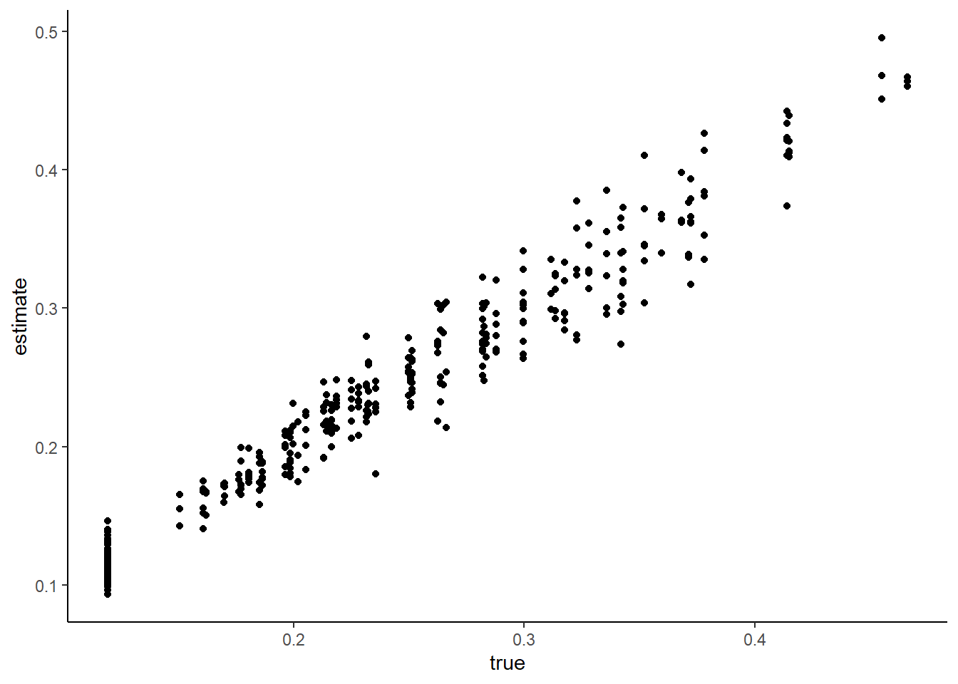

15. Write a function estimate_G_marginal(df) that returns a non-parametric estimate of the marginal transition probability matrix. Compare the estimated transition matrix and the true transition matrix by a bar plot.

# non-parametrically estimate individual transition probability
G_marginal_est <- 
  estimate_G_marginal(df = df)
check_G <- 
  data.frame(
    type = "true",
    reshape2::melt(G_marginal)
    )
check_G_est <- 
  data.frame(
    type = "estimate",
    reshape2::melt(G_marginal_est)
    )
check_G <- 
  rbind(
    check_G, 
    check_G_est
    )
check_G$variable <- 
  paste(
    check_G$Var1,
    check_G$Var2, 
    sep = "_"
    )
ggplot(
  data = check_G, 
  aes(
    x = variable, 
    y = value,
    fill = type
    )
  ) +
    geom_bar(
      stat = "identity",
      position = "dodge"
      ) +
  labs(fill = "Value") + 
  xlab("action/state/state") +
  ylab("probability") +
  theme(axis.text.x = element_blank())  + 
  theme_classic()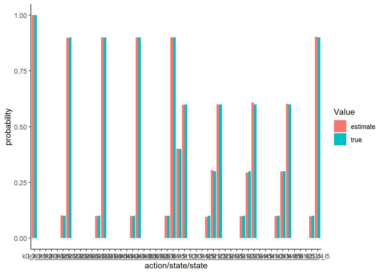

18.2 Estimate parameters

1. Vectorize the parameters as follows:

theta_1 <- 
  c(
    alpha, 
    beta, 
    eta
    )
theta_2 <- 
  c(
    kappa, 
    gamma
    )
theta <- 
  c(
    theta_1, 
    theta_2
    )

We estimate the parameters by a CCP approach.

1. Write a function estimate_theta_2_game(df) that returns the estimates of \(\kappa\) and \(\gamma\) directly from data by counting relevant events.

# estimate theta_2
theta_2_est <- 
  estimate_theta_2_game(df); 
theta_2_est

## [1] 0.09946371 0.60228274

The objective function of the minimum distance estimator based on the conditional choice probability approach is: \[ \frac{1}{N K m_s} \sum_{i = 1}^N \sum_{l = 1}^{m_s} \sum_{k = 1}^{K}\{\hat{p}_i(a_k|s_l) - p_i^{(\theta_1, \theta_2)}(a_k|s_l)\}^2, \] where \(\hat{p}_i\) is the non-parametric estimate of the marginal conditional choice probability and \(p_i^{(\theta_1, \theta_2)}\) is the marginal conditional choice probability under parameters \(\theta_1\) and \(\theta_2\) given \(\hat{p}_i\). \(a_k\) is \(k\)-th action for a firm and \(s_l\) is \(l\)-th state profile.

2. Write a function compute_CCP_objective_game(theta_1, theta_2, p_est, L, K, delta) that returns the objective function of the above minimum distance estimator given a non-parametric estimate of the conditional choice probability and \(\theta_1\) and \(\theta_2\).

# compute the objective function of the minimum distance estimator based on the CCP approach
objective <- 
  compute_CCP_objective_game(
    theta_1 = theta_1,
    theta_2 = theta_2, 
    p_marginal_est = p_marginal_est,
    A = A,
    S = S, 
    delta = delta, 
    lambda = lambda
    )
saveRDS(
  objective,
  file = "data/a8/A8_objective.rds"
  )

objective <- 
  readRDS(file = "data/a8/A8_objective.rds")
objective

## [1] 0.0003285307

3. Check the value of the objective function around the true parameter.

# label
label <- 
  c(
    "\\alpha",
    "\\beta",
    "\\eta"
    )
label <- 
  paste(
    "$",
    label,
    "$", 
    sep = ""
    )
# compute the graph
graph <- 
  foreach (
    i = 1:length(theta_1)
    ) %do% {
  theta_i <- theta_1[i]
  theta_i_list <- 
    theta_i * seq(
      0.5, 
      2,
      by = 0.2
      )
  objective_i <-
    foreach (
      j = 1:length(theta_i_list),
      .combine = "rbind"
      ) %dopar% {
               theta_ij <- theta_i_list[j]
               theta_j <- theta_1
               theta_j[i] <- theta_ij
               objective_ij <- 
                 compute_CCP_objective_game(
                   theta_j,
                   theta_2,
                   p_marginal_est, 
                   A,
                   S,
                   delta,
                   lambda
                   )
               return(objective_ij)
             }
  df_graph <- 
    data.frame(
      x = theta_i_list, 
      y = objective_i
      )
  g <- 
    ggplot(
      data = df_graph, 
      aes(
        x = x,
        y = y
        )
      ) +
    geom_point() +
    geom_vline(
      xintercept = theta_i,
      linetype = "dotted"
      ) +
    ylab("objective function") + 
    xlab(TeX(label[i])) + 
  theme_classic()
  return(g)
}
saveRDS(
  graph,
  file = "data/a8/A8_CCP_graph.rds"
  )

graph <- 
  readRDS(file = "data/a8/A8_CCP_graph.rds")
graph

## [[1]]

## 
## [[2]]

## 
## [[3]]

4. Estimate the parameters by minimizing the objective function. To keep the model to be well-defined, impose an ad hoc lower and upper bounds such that \(\alpha \in [0, 1], \beta \in [0, 5], \delta \in [0, 1]\).

lower <- 
  rep(
    0, 
    length(theta_1)
    )
upper <- c(1, 5, 0.3)
CCP_result <-
  optim(
        par = theta_1,
        fn = compute_CCP_objective_game,
        method = "L-BFGS-B",
        lower = lower,
        upper = upper,
        theta_2 = theta_2_est,
        p_marginal_est = p_marginal_est,
        A = A,
        S = S,
        delta = delta,
        lambda = lambda
        )
saveRDS(
  CCP_result, 
  file = "data/a8/A8_CCP_result.rds"
  )

CCP_result <- 
  readRDS(file = "data/a8/A8_CCP_result.rds")
CCP_result

## $par
## [1] 1.0000000 2.0205947 0.2964074
## 
## $value
## [1] 0.0003271323
## 
## $counts
## function gradient 
##       17       17 
## 
## $convergence
## [1] 0
## 
## $message
## [1] "CONVERGENCE: REL_REDUCTION_OF_F <= FACTR*EPSMCH"

compare <-
  data.frame(
    true = theta_1,
    estimate = CCP_result$par
  ); 
compare

##   true  estimate
## 1  1.0 1.0000000
## 2  2.0 2.0205947
## 3  0.3 0.2964074