Chapter 2 Introduction
2.1 What are structural models?
- An economic model is a mapping from exogenous variables (including shocks and parameters) to endogenous variables.
- This mapping is derived from a solution concept (optimality and equilibrium).
- The structural estimation approach starts from an economic model and derives an econometric model.
- The structural-form of an economic model is the equilibrium condition for the endogenous variables given the exogenous variables.
- The reduced-form of an economic model is the solution of the structural-form for the endogenous variables in terms of the exogenous variables.
2.2 Example: Linear demand and supply model
Consider a linear demand and supply model: \[\begin{align} Q_i^d = \alpha + \beta P_i + \gamma X_i + \epsilon_i \\ Q_i^s = \delta + \theta P_i + \zeta Z_i + \nu_i \end{align}\]
The parameters of the model are: \(\alpha, \beta, \gamma, \delta, \theta, \zeta\)
The observed exogenous variables are: \(X_i, Z_i\)
The unobserved exogenous variables (shocks) are: \(\epsilon_i, \nu_i\) (assume standard deviations of 1 for simplicity and mutually i.i.d.)
The endogenous variables are: \(P_i, Q_i\)
The solution concept is the market clearing condition: \[\begin{align} &Q_i^d = Q_i^s \\ &\Leftrightarrow \alpha + \beta P_i + \gamma X_i + \epsilon_i = \delta + \theta P_i + \zeta Z_i + \nu_i \end{align}\]
So far this is the structural-form of the model.
The solution is obtained by solving the endogenous variables for the exogenous variables: \[\begin{align} P_i = \frac{\alpha - \delta + \gamma X_i - \zeta Z_i + \epsilon_i - \nu_i}{\theta - \beta} \\ Q_i = \frac{\alpha \theta - \beta \delta + \theta \gamma X_i - \beta \zeta Z_i + \theta \epsilon_i - \beta \nu_i}{\theta - \beta} \end{align}\]
This is the mapping from the exogenous variables to the endogenous variables in the structural model.
This is the reduced-form of the model.
2.3 Ordinary-Least-Squares (OLS) estimation of the demand and supply model
- OLS is applied to the reduced-form of the model.
- The reduced-form model is represented by the following equation: \[\begin{align} P_i &= \pi_1 + \pi_2 X_i + \pi_3 Z_i + \sigma_1 \varepsilon_i\\ Q_i &= \pi_4 + \pi_5 X_i + \pi_6 Z_i + \sigma_2 \upsilon_i \end{align}\]
- The parameters of the reduced-form model are: \(\pi_0, \pi_1, \pi_2, \pi_3, \pi_4, \pi_5, \sigma_1, \sigma_2\) are related to the parameters of the structural-form model as follows: \[\begin{align} \pi_1 = \frac{\alpha - \delta}{\theta - \beta} \\ \pi_2 = \frac{\gamma}{\theta - \beta} \\ \pi_3 = \frac{-\zeta}{\theta - \beta} \\ \pi_4 = \frac{\alpha \theta - \beta \delta}{\theta - \beta} \\ \pi_5 = \frac{\theta \gamma}{\theta - \beta} \\ \pi_6 = \frac{- \beta \zeta}{\theta - \beta} \\ \sigma_1 = \frac{1}{\theta - \beta} \\ \sigma_2 = \frac{\sqrt{\theta^2 + \beta^2}}{\theta - \beta} \end{align}\]
- Because the right-hand side of the reduced-form model only includes exogenous variables, the OLS estimators can consistently estimate the reduced-form parameters.
- From the known 6 reduced-form parameters \(\pi_1, \pi_2, \pi_3, \pi_4, \pi_5, \pi_6\), we can recover 6 structural-form parameters \(\alpha, \beta, \gamma, \delta, \theta, \zeta\).
- This is the original idea of OLS in the context of structural estimation.
- You may be concerned that the right-hand side of the reduced-form model may include some endogenous variables — it’s just because you have not fully solved the model.
2.4 Maximum-Likelihood Estimation (MLE) of the demand and supply model
- The MLE is not very different from the above approach.
- We derive the reduced-form model.
- Then, under the distributional assumptions on the shocks, we can derive the likelihood function: \[\begin{align} L(\alpha, \beta, \gamma, \delta, \theta, \zeta) = \prod_{i=1}^n f(P_i, Q_i | X_i, Z_i) \end{align}\]
- The distributional assumptions on the shocks could be: \[\begin{align} \epsilon_i \sim N(0, 1) \\ \nu_i \sim N(0, 1) \end{align}\]
- If the structural-form parameters could be identified by the OLS estimator, then the MLE estimator should also identify them because you have the same information with a stronger distributional assumption.
2.5 Simulation-based (Simulated-Likelihood or Simulated-Method-of-Moments) methods
- In the current example, the reduced-form model is analytically derived and the likelihood function is also analytically derived.
- However, in many cases, the reduced-form model is not analytically derived and the likelihood function is not analytically derived.
- Even in this case, if we can simulate the endogenous variables solving the equilibrium condition, we can use the simulation-based methods to estimate the parameters.
- For example, by simulating shocks \(\epsilon_i\) and \(\nu_i\) from the distributional assumptions, we can simulate the endogenous variables \(P_i\) and \(Q_i\).
- Then, we can approximate the likelihood function by the empirical distribution of the simulated data.
- Or, we can find parameters that minimize the distance between the observed and simulated endogenous variables.
2.6 Two-Stage Least Squares (2SLS) estimation of the demand and supply model
- The OLS and ML estimators relied on the reduced-form model.
- The 2SLS estimator is a method to estimate the structural-form parameters of the equation of interest by representing the other equations in the reduced-form.
- Suppose that we are interested in estimating the structural-form parameters of the demand equation.
- The demand equation is: \[\begin{align} Q_i = \alpha + \beta P_i + \gamma X_i + \epsilon_i \end{align}\]
- The 2SLS estimator first runs the reduced-form model for the other equation: \[\begin{align} P_i = \pi_1 + \pi_2 X_i + \pi_3 Z_i + \sigma_1 \varepsilon_i \end{align}\]
- Then, the 2SLS estimator uses the predicted values of the endogenous variables from the reduced-form model for the supply equation to estimate the structural-form parameters of the demand equation.
- In this estimation, \(Z_i\) is used as an instrument for \(P_i\), which is an exogenous variable excluded from the demand equation.
- Instead, suppose that we are interested in estimating the structural-form parameters of the supply equation.
- The supply equation is: \[\begin{align} Q_i = \delta + \theta P_i + \zeta Z_i + \nu_i \end{align}\]
- The 2SLS estimator first runs the reduced-form model for the other equation: \[\begin{align} P_i = \pi_1 + \pi_2 X_i + \pi_3 Z_i + \sigma_1 \varepsilon_i \end{align}\]
- Then, the 2SLS estimator uses the predicted values of the endogenous variables from the reduced-form model for the demand equation to estimate the structural-form parameters of the supply equation.
- In this estimation, \(X_i\) is used as an instrument for \(P_i\), which is an exogenous variable excluded from the supply equation.
2.7 Instrumental-Variables (IV) and Generalized Method of Moments (GMM) estimation of the demand and supply model
- The IV and GMM estimators rely on another representation of the economic model.
- It relies on the moment condition of the economic model.
- In the current example, the moment condition is: \[\begin{align} & E[\epsilon_i | X_i, Z_i] = 0\\ & E[\nu_i | X_i, Z_i] = 0 \end{align}\]
- The IV and GMM estimators find the parameters that make the empirical-analogue of the moment condition zero.
- To compute the empirical-analogue of the moment condition, this time, we solve the equilibrium condition for the shocks (not for the endogenous variables).
- For example, for the demand equation, we solve the following equation for \(\epsilon_i\): \[\begin{align} \epsilon_i &= Q_i - \alpha - \beta P_i - \gamma X_i\\ \nu_i &= Q_i - \delta - \theta P_i - \zeta Z_i \end{align}\]
- Then, the right-hand side includes only observed variables and the parameters.
- Then, we can compute the implied shock from the data for candidate parameters as: \[\begin{align} \hat{\epsilon}_i &= Q_i - \hat{\alpha} - \hat{\beta} P_i - \hat{\gamma} X_i\\ \hat{\nu}_i &= Q_i - \hat{\delta} - \hat{\theta} P_i - \hat{\zeta} Z_i \end{align}\]
- Then, we can compute the empirical-analogue of the moment condition: \[\begin{align} \frac{1}{n} \sum_{i=1}^n \hat{\epsilon}_i A(Z_i, X_i) = 0\\ \frac{1}{n} \sum_{i=1}^n \hat{\nu}_i B(Z_i, X_i) = 0 \end{align}\] where \(A(Z_i, X_i)\) and \(B(Z_i, X_i)\) are some known functions of the observed variables and the parameters.
- The IV and GMM estimators find the parameters that make the empirical-analogue of the moment condition zero.
2.8 General Case
- In general, the structural-form model is represented by the following equation: \[\begin{align} f(Y_i, X_i, \epsilon_i, \theta) = 0 \end{align}\] for endogenous variables \(Y_i\), exogenous variables \(X_i\), shocks \(\epsilon_i\), and the parameters \(\theta\).
- The reduced-form model is represented by the following equation: \[\begin{align} Y_i = g(X_i, \epsilon_i, \theta) = f_1^{-1}(X_i, \epsilon_i, \theta) \end{align}\] for exogenous variables \(X_i\), shocks \(\epsilon_i\), and the parameters \(\theta\).
- We can apply OLS, ML, Simulated-Likelihood to this form.
- The moment condition is: \[\begin{align} E[h(Y_i, X_i, \theta) | X_i, \nu_i] = E[f_3^{-1}(Y_i, X_i, \theta) | X_i, \nu_i] = 0 \end{align}\]
- We can apply IV and GMM to this form.
- Thus, structural estimation is a general framework to estimate the parameters of the economic model by transforming it in either form and applying the corresponding estimation method.
2.9 Structural Estimation and Counterfactual Analysis
2.9.1 Example
Igami (2017) “Estimating the Innovator’s Dilemma: Structural Analysis of Creative Destruction in the Hard Disk Drive Industry, 1981-1998”
Question:
- Does the “Innovator’s Dilemma” (Christensen, 1997) or the delay of innovation among incumbents exist?
- Christensen argued that old winners tend to lag behind entrants even when introducing a new technology is not too difficult, with a case study of the HDD industry.
Apple’s smartphones vs. Nokia’s feature phones
Amazon vs. Borders
Kodak’s digital cameras
If it exists, what is the reason for that?
How do we empirically answer this question?
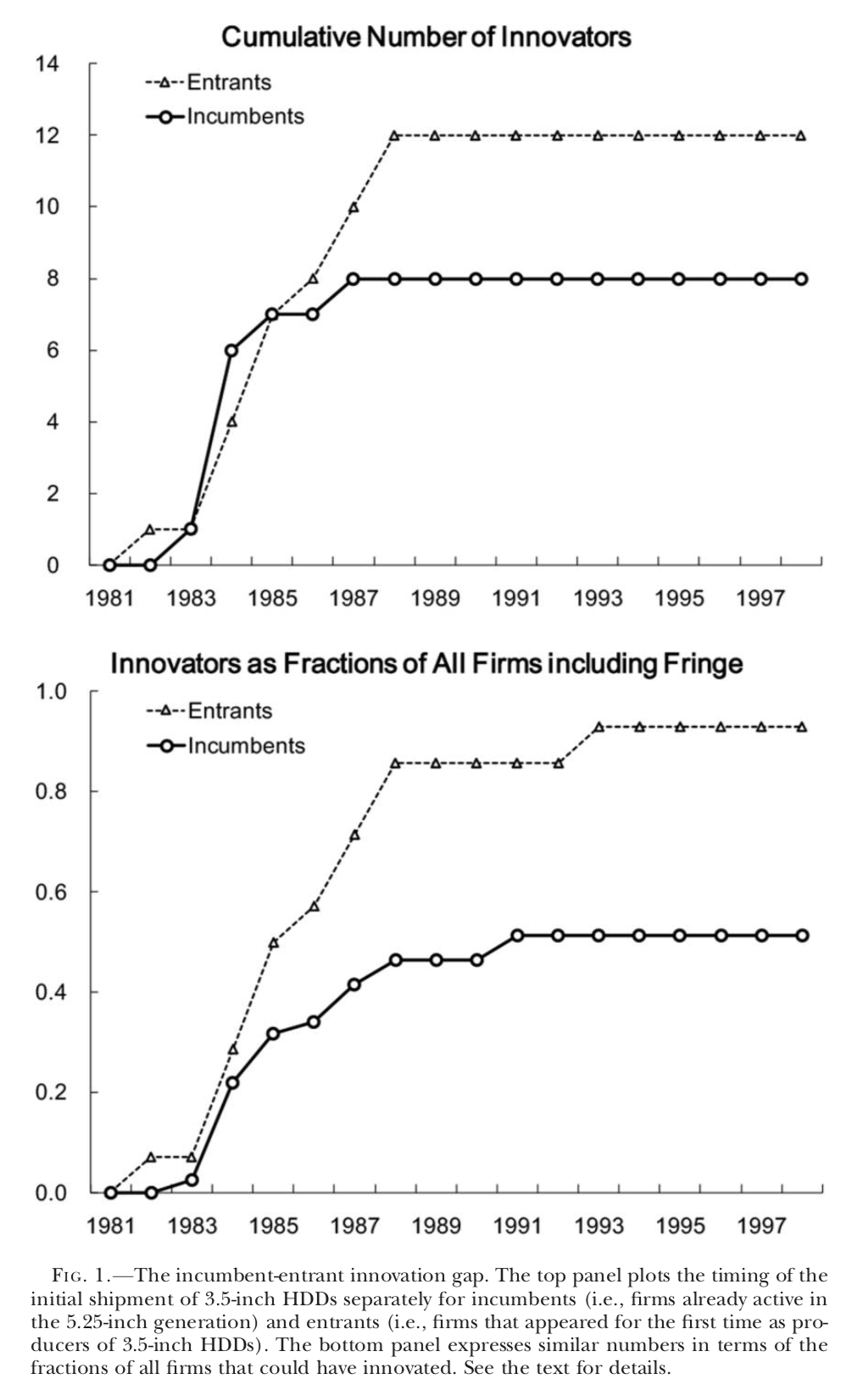
Figure 2.1: Figure 1 of Igam (2017)
Hypotheses:
Identify potentially competing hypotheses to explain the phenomenon.
- Cannibalization: Because of cannibalization, the benefits of introducing a new product are smaller for incumbents than for entrants.
- Different costs: The incumbents may have higher costs for innovation due to organizational inertia, but at the same time they may have some cost advantage due to accumulated R&D and better financial access.
- Preemption: The incumbents have additional incentive for innovation to preempt potential rivals.
- Institutional environment: The impacts of the three components differ across different institutional contexts such as the rules governing patents and market size.
Casual empiricists pick up their favorite factors to make up a story.
Serious empiricists should try to separate the contributions of each factor from data.
To do so, the author develops an economic model that explicitly incorporates the above-mentioned factors, while keeping the model parameters flexible enough to let the data tell the sign and size of the effects of each factor on innovation.
Economic model:
The time is discrete with finite horizon \(t = 1, \cdots, T\).
In each year, there is a finite number of firms indexed by \(i\).
Each firm is in one of the technological states: \[\begin{equation} s_{it} \in \{\text{old only, both, new only, potential entrant}\}, \end{equation}\] where the first two states are for incumbents (stick to the old technology or start using the new technology) and the last two states are for actual and potential entrants (enter with the new technology or stay outside the market).
In each year:
- Pre-innovation incumbent (\(s_{it} =\) old): exit or innovate by paying a sunk cost \(\kappa^{inc}\) (to be \(s_{i, t + 1} =\) both).
- Post-innovation incumbent (\(s_{it} =\) both): exit or stay to be both.
- Potential entrant (\(s_{it} =\) potential entrant): give up entry or enter with the new technology by paying a sunk cost \(\kappa^{net}\) (to be \(s_{i, t + 1} =\) new).
- Actual entrant (\(s_{it} =\) new): exit or stay to be new.
Given the industry state \(s_t = \{s_{it}\}_i\), the product market competition opens and the profit of firm \(i\), \(\pi_t(s_{it}, s_{-it})\), is realized for each active firm.
As the product market competition closes:
- Pre-innovation incumbents draw private cost shocks and make decisions: \(a_t^{pre}\).
- Observing this, post-innovation incumbents draw private cost shocks and make decisions: \(a_t^{post}\).
- Observing this, actual entrants draw private cost shocks and make decisions: \(a_t^{act}\).
- Observing this, potential entrants draw private cost shocks and make decisions: \(a_t^{pot}\).
This is a dynamic game. The equilibrium is defined by the concept of Markov-perfect equilibrium (Maskin & Tirole, 1988b).
The representation of the competing theories in the model:
- The existence of cannibalization is represented by the assumption that an incumbent maximizes the joint profits of old and new technology products.
- The size of cannibalization is captured by the shape of profit function.
- The difference in the cost of innovation is captured by the difference in the sunk costs of innovation.
- The preemptive incentive for incumbents is embodied in the dynamic optimization problem for each incumbent.
Econometric model:
The author then turns the economic model into an econometric model.
This amounts to specifying which part of the economic model is observed/known and which part is unobserved/unknown.
The author collects the data set of the HDD industry during 1977-99.
Based on the data, the author specifies the identities of active firms and their products and the technologies embodied in the products in each year to code their state variables.
Moreover, by tracking the change in the state, the author codes their action variables.
Thus, the state and action variables, \(s_t\) and \(a_t\). These are the observables.
The author does not observe:
- Profit function \(\pi_t(\cdot)\).
- Sunk cost of innovation for pre-innovation incumbents \(\kappa^{inc}\).
- Sunk cost of entry for potential entrants \(\kappa^{net}\).
- Private cost shocks.
These are the unobservables.
Among the unobservables, the profit function and sunk costs are the parameters of interest and the private cost shocks are nuisance parameters in the sense only the knowledge about the distribution of the latter is demanded.
Identification:
Can we infer the unobservables from the observables and the restrictions on the distribution of observables by the economic theory?
The profit function is identified from estimating the demand function for each firm’s product, and estimating the cost function for each firm from using their price setting behavior.
The sunk costs of innovation are identified from the conditional probability of innovation across various states. If the cost is low, the probability should be high.
Estimation:
- The identification established that in principle we can uncover the parameters of interest from observables under the restrictions of economic theory.
Finally, we apply a statistical method to the econometric model and infer the parameters of interest.
Counterfactual analysis:
- If we can uncover the parameters of interest, we can conduct comparative statics: study the change in the endogenous variables when the exogenous variables including the model parameters are set differently. In the current framework, this exercise is often called the counterfactual analysis.
What if there was no cannibalization?:
- An incumbent separately maximizes the profit from old technology and new technology instead of jointly maximizing the profits. Solve the model under this new assumption everything else being equal.
Free of cannibalization concerns, 8.95 incumbents start producing new HDDs in the first 10 years, compared with 6.30 in the baseline.
The cumulative numbers of innovators among incumbents and entrants differ only by 2.8 compared with 6.45 in the baseline.
Thus cannibalization can explain a significant part of the incumbent-entrant innovation gap.
What if there was no preemption?:
- A potential entrant ignores the incumbents’ innovations upon making entry decisions.
- Without the preemptive motives, only 6.02 incumbents would innovate in the first 10 years, compared with 6.30 in the baseline.
- The cumulative incumbent-entrant innovation gap widens to 8.91 compared with 6.45 in the baseline.
- A potential entrant ignores the incumbents’ innovations upon making entry decisions.
The sunk cost of entry is smaller for incumbents than for entrants in the baseline.
Interpretations and policy/managerial implications:
Despite the cost advantage and the preemptive motives, the speed of innovation is slower among incumbents due to the strong cannibalization effect.
Incumbents that attempt to avoid the “innovator’s dilemma” should separate the decision making between old and new sections inside the organization so that they can avoid the concern for cannibalization.
2.9.2 Recap
- The structural approach in empirical industrial organization consists of the following components:
- Research question.
- Competing hypotheses.
- Economic model.
- Econometric model.
- Identification.
- Data collection.
- Data cleaning.
- Estimation.
- Counterfactual analysis.
- Coding.
- Interpretations and policy/managerial implications.
- The goal of this course is to be familiar with the standard methodology to complete this process.
- The methodology covered in this class is mostly developed to analyze the standard framework of dynamic or oligopoly competition.
- The policy implications are centered around competition policies.
- But the basic idea can be extended to different classes of situations such as auction, matching, voting, contract, marketing, and so on.
- Note that the depth of the research question and the relevance of the policy/managerial implications are the most important parts of the research.
- Focusing on the methodology in this class is to minimize the time allocated to less important issues and maximize the attention and time to the most valuable part in future research.
- Given a research question, what kind of data is necessary to answer the question?
- Given data, what kind of research questions can you address? Which questions can be credibly answered? Which questions can be an over-stretch?
- Given a research question and data, what is the best way to answer the question? What type of problems can you avoid using the method? What is the limitation of your approach? How will you defend against possible referee comments?
- Given a result, what kinds of interpretations can you credibly derive? What kinds of interpretations can be contested by potential opponents? What kinds of contributions can you claim?
- To address these issues is necessary to publish a paper and it is necessary to be familiar with the methodology to do so.