Chapter 13 Assignment 3: Demand Function Estimation I
13.1 Simulate data
We simulate data from a discrete choice model. There are \(T\) markets and each market has \(N\) consumers. There are \(J\) products and the indirect utility of consumer \(i\) in market \(t\) for product \(j\) is: \[ u_{itj} = \beta_{it}' x_j + \alpha_{it} p_{jt} + \xi_{jt} + \epsilon_{ijt}, \] where \(\epsilon_{ijt}\) is an i.i.d. type-I extreme random variable. \(x_j\) is \(K\)-dimensional observed characteristics of the product. \(p_{jt}\) is the retail price of the product in the market.
\(\xi_{jt}\) is product-market specific fixed effect. \(p_{jt}\) can be correlated with \(\xi_{jt}\) but \(x_{jt}\)s are independent of \(\xi_{jt}\). \(j = 0\) is an outside option whose indirect utility is: \[ u_{it0} = \epsilon_{i0t}, \] where \(\epsilon_{i0t}\) is an i.i.d. type-I extreme random variable.
\(\beta_{it}\) and \(\alpha_{it}\) are different across consumers, and they are distributed as: \[ \beta_{itk} = \beta_{0k} + \sigma_k \nu_{itk}, \] \[ \alpha_{it} = - \exp(\mu + \omega \upsilon_{it}) = - \exp(\mu + \frac{\omega^2}{2}) + [- \exp(\mu + \omega \upsilon_{it}) + \exp(\mu + \frac{\omega^2}{2})] \equiv \alpha_0 + \tilde{\alpha}_{it}, \] where \(\nu_{itk}\) for \(k = 1, \cdots, K\) and \(\upsilon_{it}\) are i.i.d. standard normal random variables. \(\alpha_0\) is the mean of \(\alpha_i\) and \(\tilde{\alpha}_i\) is the deviation from the mean.
Given a choice set in the market, \(\mathcal{J}_t \cup \{0\}\), a consumer chooses the alternative that maximizes her utility: \[ q_{ijt} = 1\{u_{ijt} = \max_{k \in \mathcal{J}_t \cup \{0\}} u_{ikt}\}. \] The choice probability of product \(j\) for consumer \(i\) in market \(t\) is: \[ \sigma_{jt}(p_t, x_t, \xi_t) = \mathbb{P}\{u_{ijt} = \max_{k \in \mathcal{J}_t \cup \{0\}} u_{ikt}\}. \]
Suppose that we only observe the share data: \[ s_{jt} = \frac{1}{N} \sum_{i = 1}^N q_{ijt}, \] along with the product-market characteristics \(x_{jt}\) and the retail prices \(p_{jt}\) for \(j \in \mathcal{J}_t \cup \{0\}\) for \(t = 1, \cdots, T\). We do not observe the choice data \(q_{ijt}\) nor shocks \(\xi_{jt}, \nu_{it}, \upsilon_{it}, \epsilon_{ijt}\).
In this assignment, we consider a model with \(\xi_{jt} = 0\), i.e., the model without the unobserved fixed effects. However, the code to simulate data should be written for general \(\xi_{jt}\), so that we can use the same code in the next assignment in which we consider a model with the unobserved fixed effects.
- Set the seed, constants, and parameters of interest as follows.
# set the seed
set.seed(1)
# number of products
J <- 10
# dimension of product characteristics including the intercept
K <- 3
# number of markets
T <- 100
# number of consumers per market
N <- 500
# number of Monte Carlo
L <- 500## [1] 4.0000000 0.1836433 -0.8356286## [1] 1.5952808 0.3295078 0.8204684Generate the covariates as follows.
The product-market characteristics:
\[
x_{j1} = 1, x_{jk} \sim N(0, \sigma_x), k = 2, \cdots, K,
\]
where \(\sigma_x\) is referred to as sd_x in the code.
The product-market-specific unobserved fixed effect:
\[
\xi_{jt} = 0.
\]
The marginal cost of product \(j\) in market \(t\):
\[
c_{jt} \sim \text{logNormal}(0, \sigma_c),
\]
where \(\sigma_c\) is referred to as sd_c in the code.
The retail price:
\[
p_{jt} - c_{jt} \sim \text{logNorm}(\gamma \xi_{jt}, \sigma_p),
\]
where \(\gamma\) is referred to as price_xi and \(\sigma_p\) as sd_p in the code. This price is not the equilibrium price. We will revisit this point in a subsequent assignment.
The value of the auxiliary parameters are set as follows:
Xis the data frame such that a row contains the characteristics vector \(x_{j}\) of a product and columns are product index and observed product characteristics. The dimension of the characteristics \(K\) is specified above. Add the row of the outside option whose index is \(0\) and all the characteristics are zero.
# make product characteristics data
X <-
  matrix(
    sd_x * rnorm(J * (K - 1)),
    nrow = J
    )
X <-
  cbind(
    rep(1, J),
    X
    )
colnames(X) <- paste("x", 1:K, sep = "_")
X <-
  data.frame(
    j = 1:J,
    X
    ) %>%
  tibble::as_tibble()
# add outside option
X <-
  rbind(
    rep(0, dim(X)[2]),
    X
) ## # A tibble: 11 × 4
## j x_1 x_2 x_3
## <dbl> <dbl> <dbl> <dbl>
## 1 0 0 0 0
## 2 1 1 0.244 -0.00810
## 3 2 1 0.369 0.472
## 4 3 1 0.288 0.411
## 5 4 1 -0.153 0.297
## 6 5 1 0.756 0.459
## 7 6 1 0.195 0.391
## 8 7 1 -0.311 0.0373
## 9 8 1 -1.11 -0.995
## 10 9 1 0.562 0.310
## 11 10 1 -0.0225 -0.0281Mis the data frame such that a row contains the price \(\xi_{jt}\), marginal cost \(c_{jt}\), and price \(p_{jt}\). After generating the variables, drop1 - prop_jtproducts from each market usingdplyr::sample_fracfunction. The variation in the available products is important for the identification of the distribution of consumer-level unobserved heterogeneity. Add the row of the outside option to each market whose index is \(0\) and all the variables take value zero.
# make market-product data
M <-
  expand.grid(
    j = 1:J,
    t = 1:T
    ) %>%
  tibble::as_tibble() %>%
  dplyr::mutate(
    xi = 0,
    c = exp(sd_c * rnorm(J*T)),
    p = exp(price_xi * xi + sd_p * rnorm(J*T)) + c
  )
M <-
  M %>%
  dplyr::group_by(t) %>%
  dplyr::sample_frac(prop_jt) %>%
  dplyr::ungroup()
# add outside option
outside <-
  data.frame(
    j = 0,
    t = 1:T,
    xi = 0,
    c = 0,
    p = 0
    )
M <-
  rbind(
    M,
    outside
    ) %>%
  dplyr::arrange(
    t,
    j
)## # A tibble: 700 × 5
## j t xi c p
## <dbl> <int> <dbl> <dbl> <dbl>
## 1 0 1 0 0 0
## 2 2 1 0 0.929 1.97
## 3 3 1 0 0.976 1.91
## 4 4 1 0 1.02 2.05
## 5 6 1 0 0.995 1.98
## 6 7 1 0 1.02 1.98
## 7 8 1 0 0.997 1.99
## 8 0 2 0 0 0
## 9 1 2 0 0.980 1.97
## 10 4 2 0 1.04 2.04
## # ℹ 690 more rows- Generate the consumer-level heterogeneity.
Vis the data frame such that a row contains the vector of shocks to consumer-level heterogeneity, \((\nu_{i}', \upsilon_i)\). They are all i.i.d. standard normal random variables.
# make consumer-market data
V <-
  matrix(
    rnorm(N * T * (K + 1)),
    nrow = N * T
    )
colnames(V) <- c(paste("v_x", 1:K, sep = "_"), "v_p")
V <-
  data.frame(
    expand.grid(
      i = 1:N,
      t = 1:T
      ),
    V
    ) %>%
tibble::as_tibble()## # A tibble: 50,000 × 6
## i t v_x_1 v_x_2 v_x_3 v_p
## <int> <int> <dbl> <dbl> <dbl> <dbl>
## 1 1 1 1.32 -0.0670 -0.758 -0.590
## 2 2 1 0.930 1.34 1.16 0.0684
## 3 3 1 1.08 0.768 -0.725 -0.130
## 4 4 1 -0.300 0.156 -0.641 -0.896
## 5 5 1 1.04 1.17 -0.224 1.31
## 6 6 1 0.709 -0.286 0.948 1.15
## 7 7 1 -1.27 0.193 -0.212 -0.156
## 8 8 1 -0.932 -0.780 1.49 -0.362
## 9 9 1 1.37 -0.205 0.594 -0.998
## 10 10 1 -0.461 -0.834 0.221 -1.62
## # ℹ 49,990 more rows- Join
X,M,Vusingdplyr::left_joinand name itdf.dfis the data frame such that a row contains variables for a consumer about a product that is available in a market.
# make choice data
df <-
  expand.grid(
    t = 1:T,
    i = 1:N,
    j = 0:J
    ) %>%
  tibble::as_tibble() %>%
  dplyr::left_join(
    V,
    by = c("i", "t")
    ) %>%
  dplyr::left_join(
    X,
    by = c("j")
    ) %>%
  dplyr::left_join(
    M,
    by = c("j", "t")
    ) %>%
  dplyr::filter(!is.na(p)) %>%
  dplyr::arrange(
    t,
    i,
    j
)## # A tibble: 350,000 × 13
## t i j v_x_1 v_x_2 v_x_3 v_p x_1 x_2 x_3 xi
## <int> <int> <dbl> <dbl> <dbl> <dbl> <dbl> <dbl> <dbl> <dbl> <dbl>
## 1 1 1 0 1.32 -0.0670 -0.758 -0.590 0 0 0 0
## 2 1 1 2 1.32 -0.0670 -0.758 -0.590 1 0.369 0.472 0
## 3 1 1 3 1.32 -0.0670 -0.758 -0.590 1 0.288 0.411 0
## 4 1 1 4 1.32 -0.0670 -0.758 -0.590 1 -0.153 0.297 0
## 5 1 1 6 1.32 -0.0670 -0.758 -0.590 1 0.195 0.391 0
## 6 1 1 7 1.32 -0.0670 -0.758 -0.590 1 -0.311 0.0373 0
## 7 1 1 8 1.32 -0.0670 -0.758 -0.590 1 -1.11 -0.995 0
## 8 1 2 0 0.930 1.34 1.16 0.0684 0 0 0 0
## 9 1 2 2 0.930 1.34 1.16 0.0684 1 0.369 0.472 0
## 10 1 2 3 0.930 1.34 1.16 0.0684 1 0.288 0.411 0
## # ℹ 349,990 more rows
## # ℹ 2 more variables: c <dbl>, p <dbl>- Draw a vector of preference shocks
ewhose length is the same as the number of rows ofdf.
## [1] 0.32969177 -1.03771238 1.41496338 5.02048718 -0.01302806 0.57956001- Write a function
compute_indirect_utility(df, beta, sigma, mu, omega)that returns a vector whose element is the mean indirect utility of a product for a consumer in a market. The output should have the same length with \(e\).
##             u
## [1,] 0.000000
## [2,] 3.681882
## [3,] 3.807728
## [4,] 3.779036
## [5,] 3.764454
## [6,] 4.193113- Write a function
compute_choice(X, M, V, e, beta, sigma, mu, omega)that first constructdffromX,M,V, second callcompute_indirect_utilityto obtain the vector of mean indirect utilitiesu, third compute the choice vectorqbased on the vector of mean indirect utilities ande, and finally return the data frame to whichuandqare added as columns.
## # A tibble: 350,000 × 16
##        t     i     j v_x_1   v_x_2  v_x_3     v_p   x_1    x_2     x_3    xi
##    <int> <int> <dbl> <dbl>   <dbl>  <dbl>   <dbl> <dbl>  <dbl>   <dbl> <dbl>
##  1     1     1     0 1.32  -0.0670 -0.758 -0.590      0  0      0          0
##  2     1     1     2 1.32  -0.0670 -0.758 -0.590      1  0.369  0.472      0
##  3     1     1     3 1.32  -0.0670 -0.758 -0.590      1  0.288  0.411      0
##  4     1     1     4 1.32  -0.0670 -0.758 -0.590      1 -0.153  0.297      0
##  5     1     1     6 1.32  -0.0670 -0.758 -0.590      1  0.195  0.391      0
##  6     1     1     7 1.32  -0.0670 -0.758 -0.590      1 -0.311  0.0373     0
##  7     1     1     8 1.32  -0.0670 -0.758 -0.590      1 -1.11  -0.995      0
##  8     1     2     0 0.930  1.34    1.16   0.0684     0  0      0          0
##  9     1     2     2 0.930  1.34    1.16   0.0684     1  0.369  0.472      0
## 10     1     2     3 0.930  1.34    1.16   0.0684     1  0.288  0.411      0
## # ℹ 349,990 more rows
## # ℹ 5 more variables: c <dbl>, p <dbl>, u <dbl>, e <dbl>, q <dbl>## t i j v_x_1
## Min. : 1.00 Min. : 1.0 Min. : 0.000 Min. :-4.302781
## 1st Qu.: 25.75 1st Qu.:125.8 1st Qu.: 2.000 1st Qu.:-0.683141
## Median : 50.50 Median :250.5 Median : 5.000 Median : 0.001562
## Mean : 50.50 Mean :250.5 Mean : 4.791 Mean :-0.002669
## 3rd Qu.: 75.25 3rd Qu.:375.2 3rd Qu.: 8.000 3rd Qu.: 0.669657
## Max. :100.00 Max. :500.0 Max. :10.000 Max. : 3.809895
## v_x_2 v_x_3 v_p x_1
## Min. :-4.542122 Min. :-3.957618 Min. :-4.218131 Min. :0.0000
## 1st Qu.:-0.680086 1st Qu.:-0.673321 1st Qu.:-0.671449 1st Qu.:1.0000
## Median : 0.002374 Median : 0.004941 Median : 0.001083 Median :1.0000
## Mean :-0.000890 Mean : 0.003589 Mean :-0.002011 Mean :0.8571
## 3rd Qu.: 0.673194 3rd Qu.: 0.676967 3rd Qu.: 0.671318 3rd Qu.:1.0000
## Max. : 4.313621 Max. : 4.244194 Max. : 4.017246 Max. :1.0000
## x_2 x_3 xi c
## Min. :-1.10735 Min. :-0.9947 Min. :0 Min. :0.0000
## 1st Qu.:-0.15269 1st Qu.: 0.0000 1st Qu.:0 1st Qu.:0.9404
## Median : 0.19492 Median : 0.2970 Median :0 Median :0.9841
## Mean : 0.05989 Mean : 0.1128 Mean :0 Mean :0.8560
## 3rd Qu.: 0.36916 3rd Qu.: 0.3911 3rd Qu.:0 3rd Qu.:1.0260
## Max. : 0.75589 Max. : 0.4719 Max. :0 Max. :1.2099
## p u e q
## Min. :0.000 Min. :-190.479 Min. :-2.6364 Min. :0.0000
## 1st Qu.:1.913 1st Qu.: -2.177 1st Qu.:-0.3301 1st Qu.:0.0000
## Median :1.981 Median : 0.000 Median : 0.3635 Median :0.0000
## Mean :1.712 Mean : -1.291 Mean : 0.5763 Mean :0.1429
## 3rd Qu.:2.039 3rd Qu.: 1.978 3rd Qu.: 1.2418 3rd Qu.:0.0000
## Max. :2.293 Max. : 10.909 Max. :14.0966 Max. :1.0000- Write a function
compute_share(X, M, V, e, beta, sigma, mu, omega)that first constructdffromX,M,V, second callcompute_choiceto obtain a data frame withuandq, third compute the share of each product at each marketsand the log difference in the share from the outside option, \(\ln(s_{jt}/s_{0t})\), denoted byy, and finally return the data frame that is summarized at the product-market level, dropped consumer-level variables, and addedsandy.
## # A tibble: 700 × 11
##        t     j   x_1    x_2      x_3    xi     c     p     q     s       y
##    <int> <dbl> <dbl>  <dbl>    <dbl> <dbl> <dbl> <dbl> <dbl> <dbl>   <dbl>
##  1     1     0     0  0      0           0 0      0      144 0.288  0
##  2     1     2     1  0.369  0.472       0 0.929  1.97    47 0.094 -1.12
##  3     1     3     1  0.288  0.411       0 0.976  1.91    37 0.074 -1.36
##  4     1     4     1 -0.153  0.297       0 1.02   2.05    35 0.07  -1.41
##  5     1     6     1  0.195  0.391       0 0.995  1.98    60 0.12  -0.875
##  6     1     7     1 -0.311  0.0373      0 1.02   1.98    44 0.088 -1.19
##  7     1     8     1 -1.11  -0.995       0 0.997  1.99   133 0.266 -0.0795
##  8     2     0     0  0      0           0 0      0      170 0.34   0
##  9     2     1     1  0.244 -0.00810     0 0.980  1.97    84 0.168 -0.705
## 10     2     4     1 -0.153  0.297       0 1.04   2.04    35 0.07  -1.58
## # ℹ 690 more rows## t j x_1 x_2
## Min. : 1.00 Min. : 0.000 Min. :0.0000 Min. :-1.10735
## 1st Qu.: 25.75 1st Qu.: 2.000 1st Qu.:1.0000 1st Qu.:-0.15269
## Median : 50.50 Median : 5.000 Median :1.0000 Median : 0.19492
## Mean : 50.50 Mean : 4.791 Mean :0.8571 Mean : 0.05989
## 3rd Qu.: 75.25 3rd Qu.: 8.000 3rd Qu.:1.0000 3rd Qu.: 0.36916
## Max. :100.00 Max. :10.000 Max. :1.0000 Max. : 0.75589
## x_3 xi c p
## Min. :-0.9947 Min. :0 Min. :0.0000 Min. :0.000
## 1st Qu.: 0.0000 1st Qu.:0 1st Qu.:0.9404 1st Qu.:1.913
## Median : 0.2970 Median :0 Median :0.9841 Median :1.981
## Mean : 0.1128 Mean :0 Mean :0.8560 Mean :1.712
## 3rd Qu.: 0.3911 3rd Qu.:0 3rd Qu.:1.0260 3rd Qu.:2.039
## Max. : 0.4719 Max. :0 Max. :1.2099 Max. :2.293
## q s y
## Min. : 26.00 Min. :0.0520 Min. :-1.89354
## 1st Qu.: 43.00 1st Qu.:0.0860 1st Qu.:-1.35812
## Median : 52.00 Median :0.1040 Median :-1.16644
## Mean : 71.43 Mean :0.1429 Mean :-0.99214
## 3rd Qu.: 73.00 3rd Qu.:0.1460 3rd Qu.:-0.81801
## Max. :195.00 Max. :0.3900 Max. : 0.0519613.2 Estimate the parameters
- Estimate the parameters assuming there is no consumer-level heterogeneity, i.e., by assuming:
\[
\ln \frac{s_{jt}}{s_{0t}} = \beta' x_{jt} + \alpha p_{jt}.
\]
This can be implemented using
lmfunction. Print out the estimate results.
##
## Call:
## lm(formula = y ~ -1 + x_1 + x_2 + x_3 + p, data = df_share)
##
## Residuals:
##      Min       1Q   Median       3Q      Max
## -0.57415 -0.09781  0.00000  0.10491  0.51149
##
## Coefficients:
##     Estimate Std. Error t value Pr(>|t|)
## x_1  1.20614    0.18150   6.646 6.10e-11 ***
## x_2  0.21995    0.02841   7.741 3.49e-14 ***
## x_3 -0.92818    0.03364 -27.589  < 2e-16 ***
## p   -1.12982    0.09086 -12.435  < 2e-16 ***
## ---
## Signif. codes:  0 '***' 0.001 '**' 0.01 '*' 0.05 '.' 0.1 ' ' 1
##
## Residual standard error: 0.1677 on 696 degrees of freedom
## Multiple R-squared:  0.9778, Adjusted R-squared:  0.9777
## F-statistic:  7678 on 4 and 696 DF,  p-value: < 2.2e-16
We estimate the model using simulated share.
When optimizing an objective function that uses the Monte Carlo simulation, it is important to keep the realizations of the shocks the same across the evaluations of the objective function. If the realization of the shocks differ across the objective function evaluations, the optimization algorithm will not converge because it cannot distinguish the change in the value of the objective function due to the difference in the parameters and the difference in the realized shocks.
The best practice to avoid this problem is to generate the shocks outside the optimization algorithm as in the current case. If the size of the shocks can be too large to store in the memory, the second best practice is to make sure to set the seed inside the optimization algorithm so that the realized shocks are the same across function evaluations.
- For this reason, we first draw Monte Carlo consumer-level heterogeneity
V_mcmcand Monte Carlo preference shockse_mcmc. The number of simulations isL. This does not have to be the same with the actual number of consumersN.
# mixed logit estimation
## draw mcmc V
V_mcmc <-
  matrix(
    rnorm(L * T * (K + 1)),
    nrow = L * T
    )
colnames(V_mcmc) <- c(paste("v_x", 1:K, sep = "_"), "v_p")
V_mcmc <-
  data.frame(
    expand.grid(
      i = 1:L,
      t = 1:T
      ),
    V_mcmc
    ) %>%
tibble::as_tibble() ## # A tibble: 50,000 × 6
## i t v_x_1 v_x_2 v_x_3 v_p
## <int> <int> <dbl> <dbl> <dbl> <dbl>
## 1 1 1 -0.715 -0.798 -0.548 1.09
## 2 2 1 0.0243 -0.943 -1.88 0.471
## 3 3 1 -0.183 0.660 0.669 1.45
## 4 4 1 0.0207 3.36 -0.363 1.58
## 5 5 1 -1.94 0.221 1.02 0.943
## 6 6 1 0.876 -0.636 0.0432 0.324
## 7 7 1 1.96 -0.195 -0.0950 1.39
## 8 8 1 1.11 0.571 1.77 0.497
## 9 9 1 1.45 0.154 1.96 0.740
## 10 10 1 -1.00 -0.413 0.0542 -0.469
## # ℹ 49,990 more rows## draw mcmc e
df_mcmc <-
expand.grid(
t = 1:T,
i = 1:L,
j = 0:J
) %>%
tibble::as_tibble() %>%
dplyr::left_join(
V_mcmc,
by = c("i", "t")
) %>%
dplyr::left_join(
X,
by = c("j")
) %>%
dplyr::left_join(
M,
by = c("j", "t")
) %>%
dplyr::filter(!is.na(p)) %>%
dplyr::arrange(
t,
i,
j
)
# draw idiosyncratic shocks
e_mcmc <- evd::rgev(dim(df_mcmc)[1])## [1] 0.265602821 0.652183731 -0.006127627 -0.317288366 3.145022297
## [6] -1.277026910- Use
compute_shareto check the simulated share at the true parameter using the Monte Carlo shocks. Remember that the number of consumers should be set atLinstead ofN.
## # A tibble: 700 × 11
##        t     j   x_1    x_2      x_3    xi     c     p     q     s      y
##    <int> <dbl> <dbl>  <dbl>    <dbl> <dbl> <dbl> <dbl> <dbl> <dbl>  <dbl>
##  1     1     0     0  0      0           0 0      0      171 0.342  0
##  2     1     2     1  0.369  0.472       0 0.929  1.97    46 0.092 -1.31
##  3     1     3     1  0.288  0.411       0 0.976  1.91    37 0.074 -1.53
##  4     1     4     1 -0.153  0.297       0 1.02   2.05    38 0.076 -1.50
##  5     1     6     1  0.195  0.391       0 0.995  1.98    38 0.076 -1.50
##  6     1     7     1 -0.311  0.0373      0 1.02   1.98    52 0.104 -1.19
##  7     1     8     1 -1.11  -0.995       0 0.997  1.99   118 0.236 -0.371
##  8     2     0     0  0      0           0 0      0      194 0.388  0
##  9     2     1     1  0.244 -0.00810     0 0.980  1.97    62 0.124 -1.14
## 10     2     4     1 -0.153  0.297       0 1.04   2.04    37 0.074 -1.66
## # ℹ 690 more rows- Vectorize the parameters to a vector
thetabecauseoptimrequires the maximiand to be a vector.
## [1]  4.0000000  0.1836433 -0.8356286  1.5952808  0.3295078  0.8204684  0.5000000
## [8] 1.0000000- Write a function
compute_nlls_objective_a3(theta, df_share, X, M, V_mcmc, e_mcmc)that first computes the simulated share and then compute the mean-squared error between the share data.
## [1] 0.0004815657- Draw a graph of the objective function that varies each parameter from 0.5, 0.6, \(\cdots\), 1.5 of the true value. First try with the actual shocks
Vandeand then try with the Monte Carlo shocksV_mcmcande_mcmc. You will some of the graph does not look good with the Monte Carlo shocks. It will cause the approximation error.
Because this takes time, you may want to parallelize the computation using %dopar functionality of foreach loop. To do so, first install doParallel package and then load it and register the workers as follows:
This automatically detect the number of cores available at your computer and registers them as the workers. Then, you only have to change %do% to %dopar in the foreach loop as follows:
## [[1]]
## [1] 2
##
## [[2]]
## [1] 4
##
## [[3]]
## [1] 6
##
## [[4]]
## [1] 8
In windows, you may have to explicitly pass packages, functions, and data to the worker by using .export and .packages options as follows:
temp_func <-
  function(x) {
    y <- 2 * x
    return(y)
}
foreach (
  i = 1:4,
  .export = "temp_func",
  .packages = "magrittr"
  ) %dopar% {
    # this part is parallelized
    y <- temp_func(i)
    return(y)
}
## Warning in e$fun(obj, substitute(ex), parent.frame(), e$data): already
## exporting variable(s): temp_func## [[1]]
## [1] 2
##
## [[2]]
## [1] 4
##
## [[3]]
## [1] 6
##
## [[4]]
## [1] 8If you have called a function in a package in this way dplyr::mutate, then you will not have to pass dplyr by .packages option. This is one of the reasons why I prefer to explicitly call the package every time I call a function. If you have compiled your functions in a package, you will just have to pass the package as follows:
# this function is compiled in the package EmpiricalIO
# temp_func <- function(x) {
#   y <- 2 * x
#   return(y)
# }
foreach (
  i = 1:4,
  .packages = c(
    "EmpiricalIO",
    "magrittr")
  ) %dopar% {
    # this part is parallelized
    y <- temp_func(i)
    return(y)
}
## [[1]]
## [1] 2
##
## [[2]]
## [1] 4
##
## [[3]]
## [1] 6
##
## [[4]]
## [1] 8The graphs with the true shocks:
## [[1]]
##
## [[2]]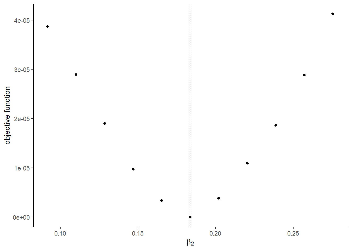
##
## [[3]]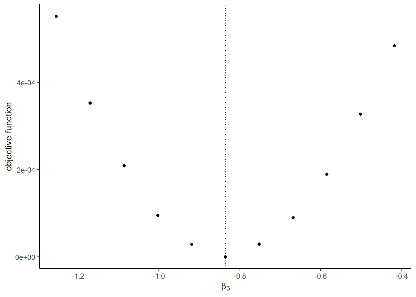
##
## [[4]]
##
## [[5]]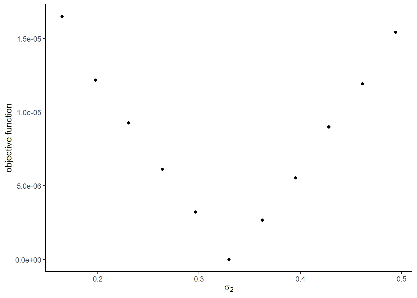
##
## [[6]]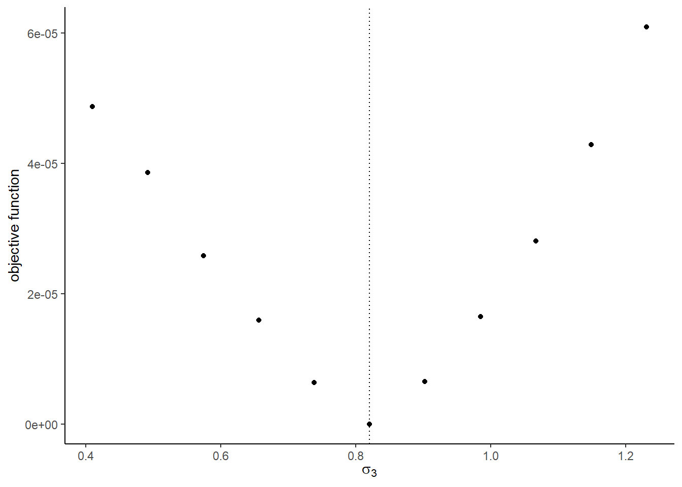
##
## [[7]]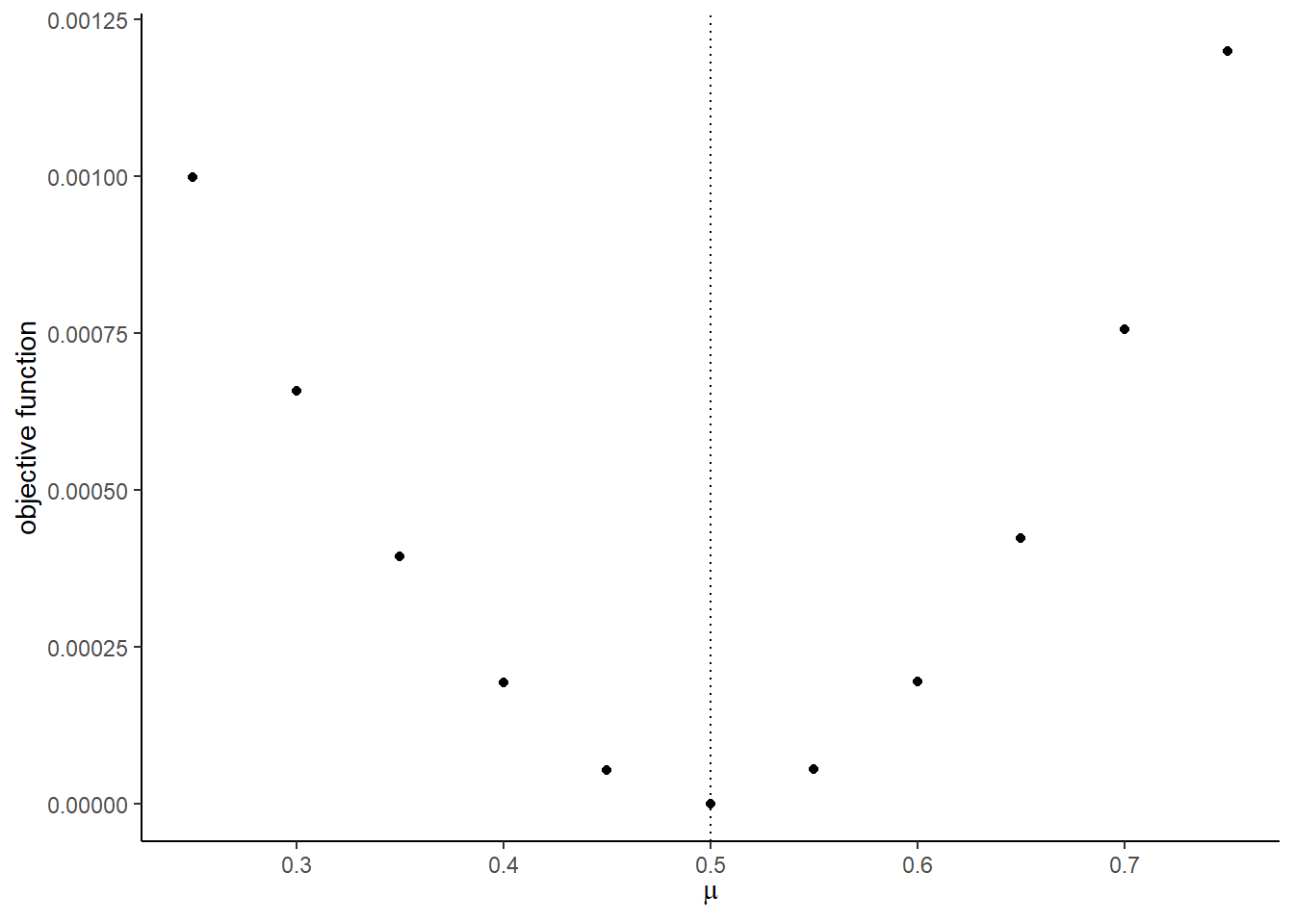
##
## [[8]]
The graphs with the Monte Carlo shocks:
## [[1]]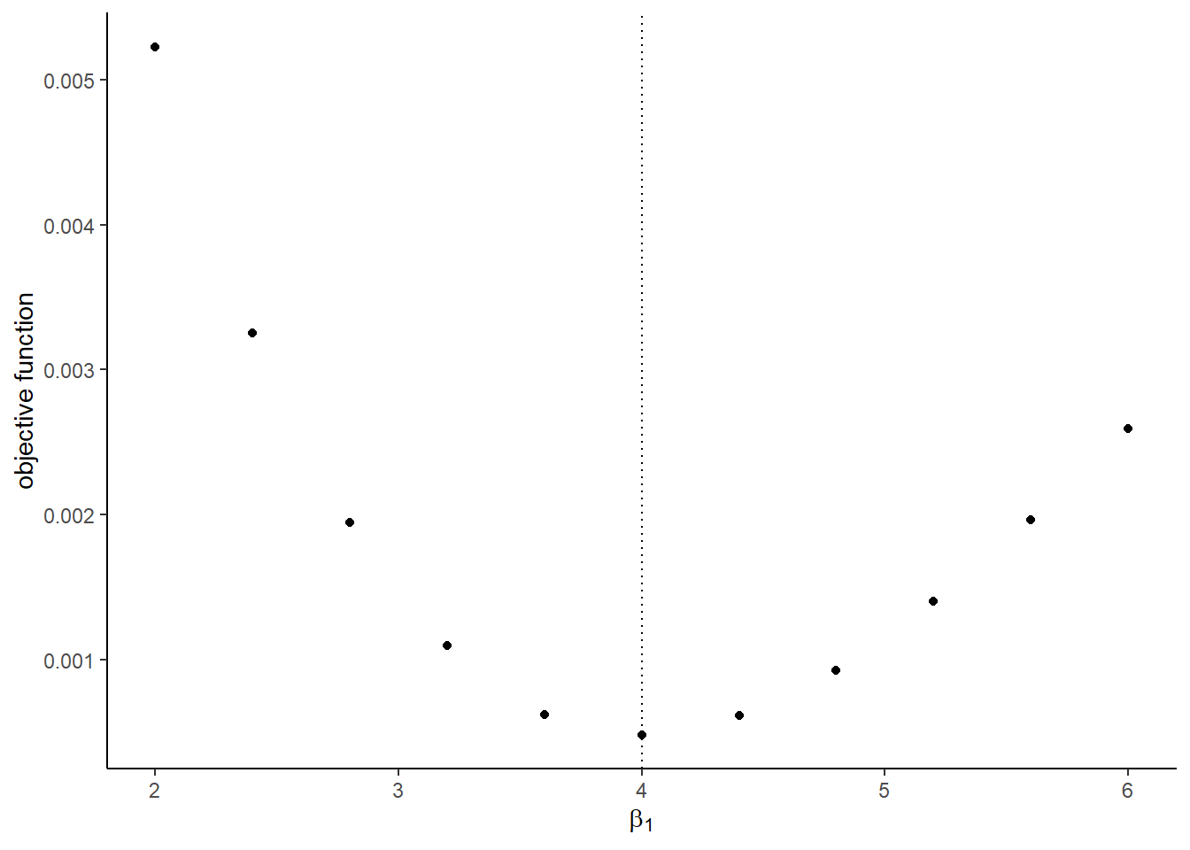
##
## [[2]]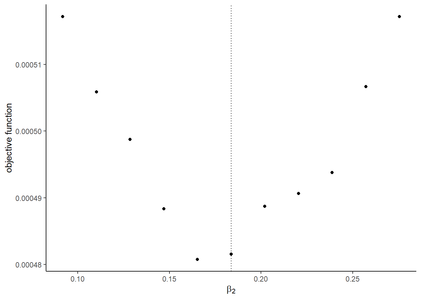
##
## [[3]]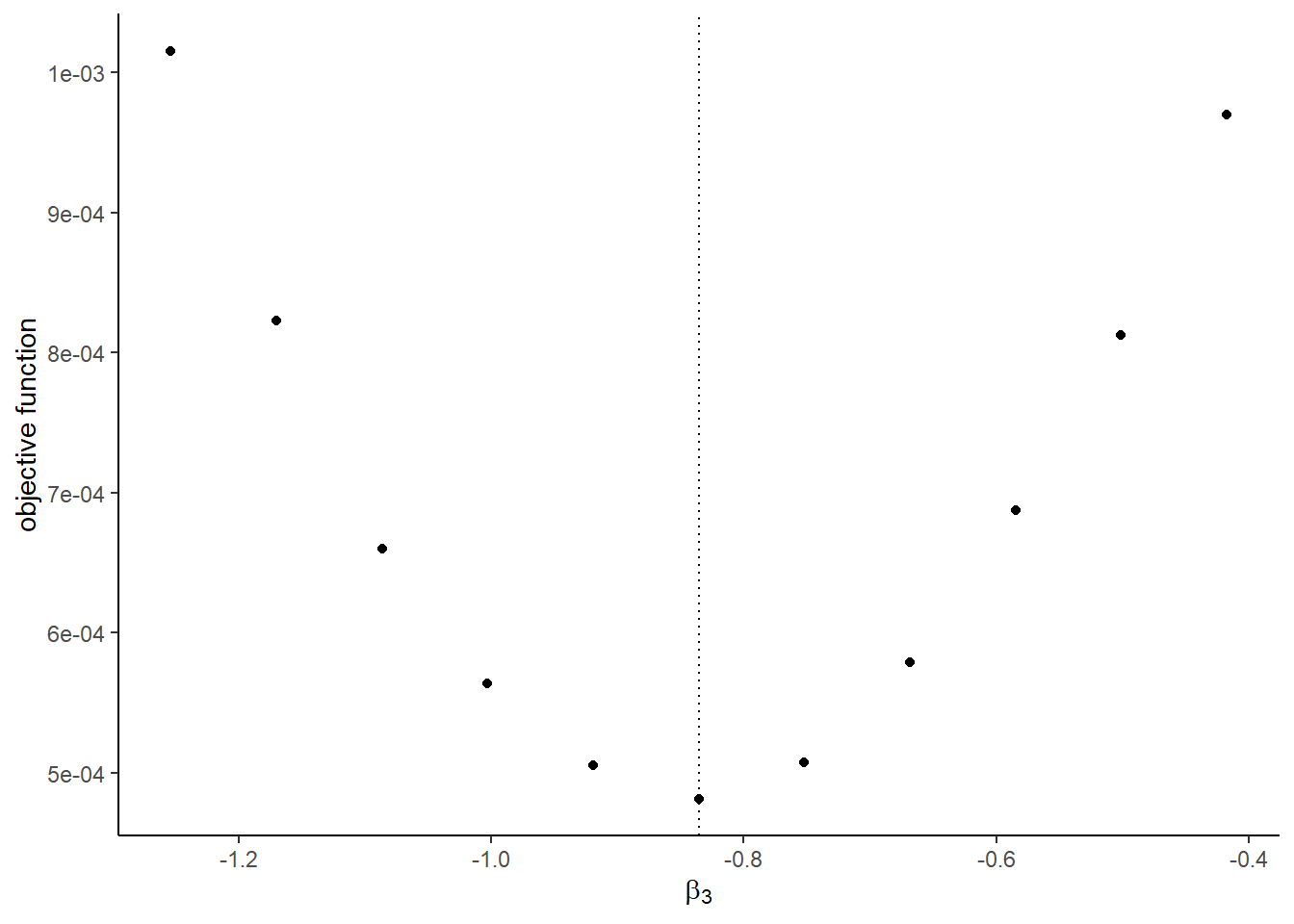
##
## [[4]]
##
## [[5]]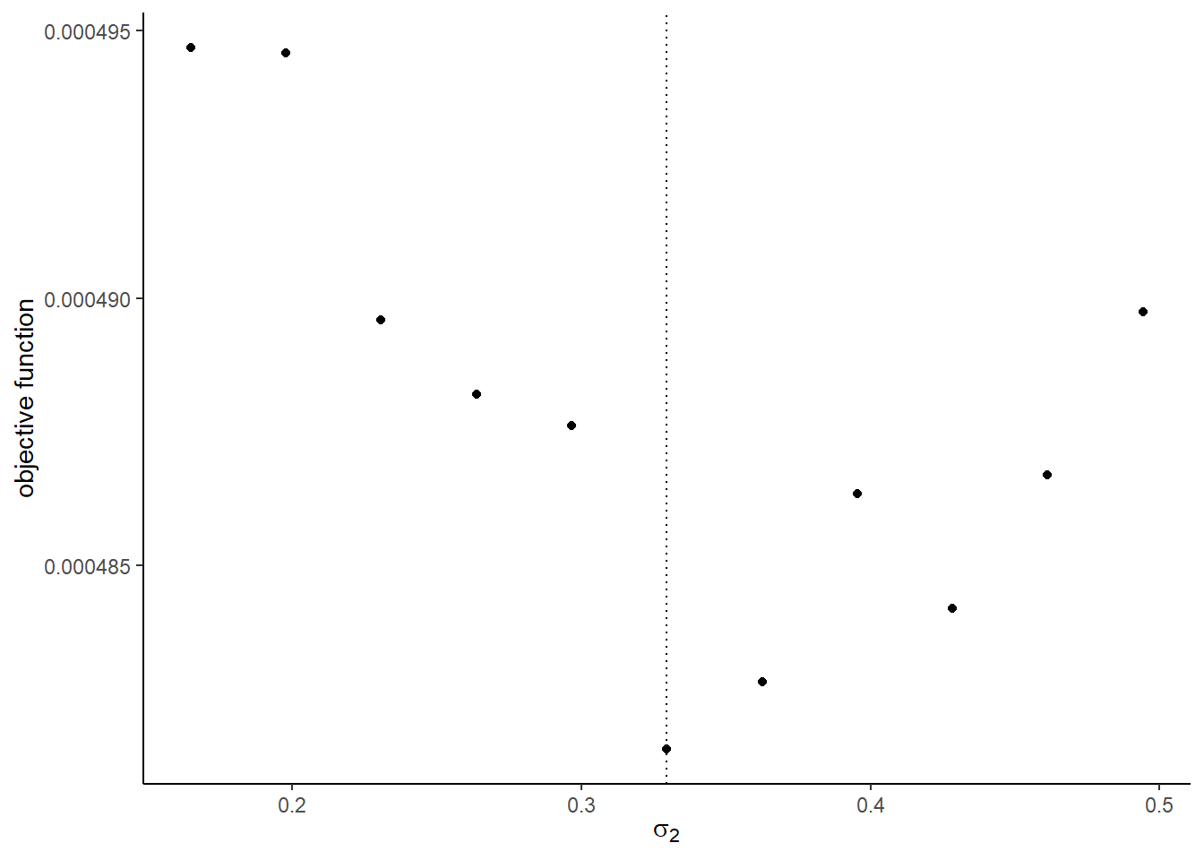
##
## [[6]]
##
## [[7]]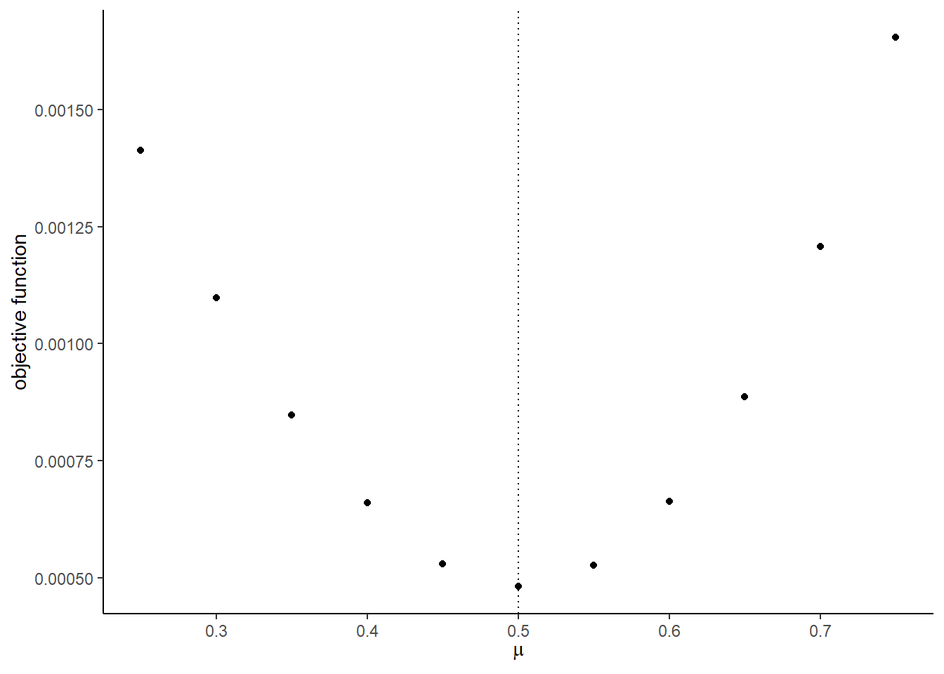
##
## [[8]]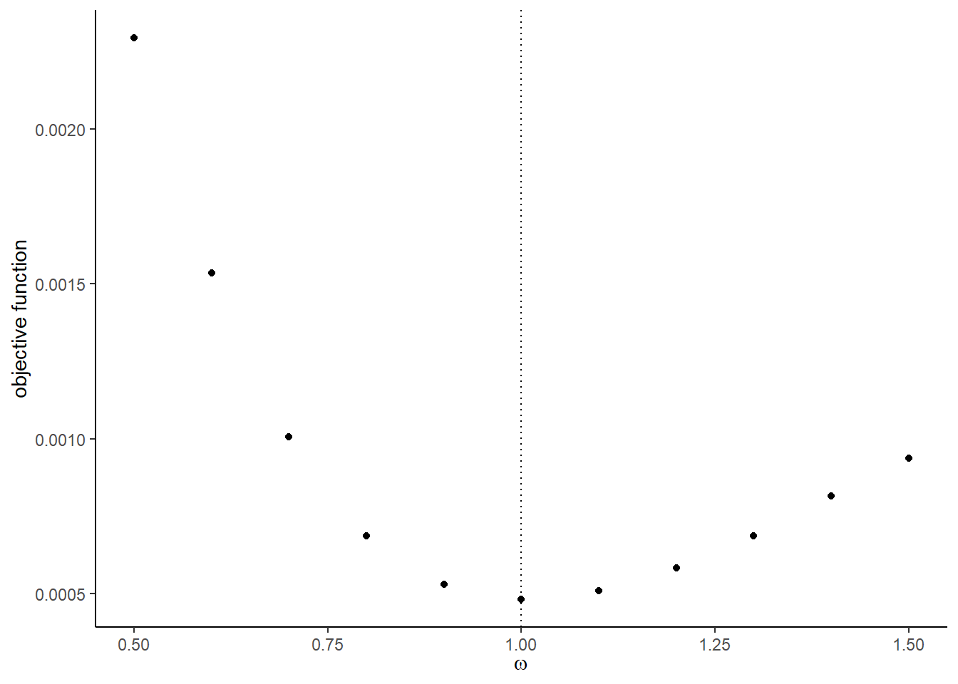
- Use
optimto find the minimizer of the objective function usingNelder-Meadmethod. You can start from the true parameter values. Compare the estimates with the true parameters.
## $par
## [1]  3.9907237  0.1778582 -0.8244977  1.5326774  0.3602383  0.9336009  0.4883030
## [8]  1.0462494
##
## $value
## [1] 0.0004678286
##
## $counts
## function gradient
##      237       NA
##
## $convergence
## [1] 0
##
## $message
## NULL
## true estimates
## 1 4.0000000 3.9907237
## 2 0.1836433 0.1778582
## 3 -0.8356286 -0.8244977
## 4 1.5952808 1.5326774
## 5 0.3295078 0.3602383
## 6 0.8204684 0.9336009
## 7 0.5000000 0.4883030
## 8 1.0000000 1.0462494