Chapter 19 Assignment 9: Auction

19.1 Simulate data

We simulate bid data from a second- and first-price sealed bid auctions.

First, we draw bid data from a second-price sealed bid auctions. Suppose that for each auction \(t = 1, \cdots, T\), there are \(i = 2, \cdots, n_t\) potential bidders. At each auction, an auctioneer allocates one item and sets the reserve price at \(r_t\). When the signal for bidder \(i\) in auction \(t\) is \(x_{it}\), her expected value of the item is \(x_{it}\). A signal \(x_{it}\) is drawn from an i.i.d. beta distribution \(B(\alpha, \beta)\). Let \(F_X(\cdot; \alpha, \beta)\) be its distribution and \(f_X(\cdot; \alpha, \beta)\) be the density. A reserve is set at 0.2. \(n_t\) is drawn from a Poisson distribution with mean \(\lambda\). If \(n_t = 1\), replace with \(n_t = 2\) to ensure at least two potential bidders. An equilibrium strategy is such that a bidder participates and bids \(\beta(x) = x\) if \(x \ge r_t\) and does not participate otherwise.

Set the constants and parameters as follows:

# set seed
set.seed(1)
# number of auctions
T <- 100
# parameter of value distribution
alpha <- 2
beta <- 2
# prameters of number of potential bidders
lambda <- 10

Draw a vector of valuations and reservation prices.

# number of bidders
N <- 
  rpois(
    T, 
    lambda
    )
N <- 
  ifelse(
    N == 1, 
    2, 
    N
    )
# draw valuations
valuation <-
  foreach (
    tt = 1:T, 
    .combine = "rbind"
    ) %do% {
    n_t <- N[tt]
    header <- 
      expand.grid(
        t = tt,
        i = 1:n_t
        ) 
    return(header)
  }
valuation <- 
  valuation %>%
  tibble::as_tibble() %>%
  dplyr::mutate(x = 
                  rbeta(
                    length(i),
                    alpha,beta
                    )
                )
ggplot(
  valuation, 
  aes(x = x)
  ) + 
  geom_histogram(
    fill = "steelblue",
    alpha = 0.8
    ) + 
  theme_classic()

## `stat_bin()` using `bins = 30`. Pick better value with
## `binwidth`.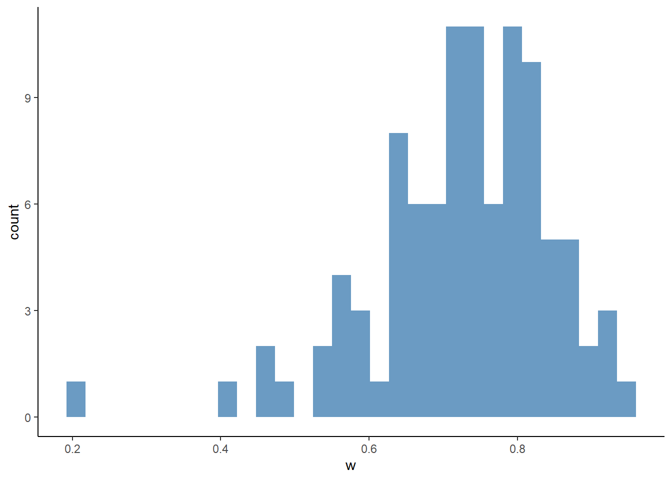

# draw reserve prices
reserve <- 0.2
reserve <- 
  tibble::tibble(
    t = 1:T, 
    r = reserve
    )

Write a function compute_winning_bids_second(valuation, reserve) that returns a winning bid from each second-price auction. It returns nothing for an auction in which no bid was above the reserve price. In the output, t refers to the auction index, m to the number of actual bidders, r to the reserve price, and w to the winning bid.

# compute winning bids from second-price auction
df_second_w <-
  compute_winning_bids_second(
    valuation = valuation, 
    reserve = reserve
    )
df_second_w

## # A tibble: 100 × 5
##        t     n     m     r     w
##    <int> <int> <int> <dbl> <dbl>
##  1     1     8     8   0.2 0.637
##  2     2    10    10   0.2 0.647
##  3     3     7     5   0.2 0.484
##  4     4    11     8   0.2 0.804
##  5     5    14    12   0.2 0.920
##  6     6    12    11   0.2 0.942
##  7     7    11     9   0.2 0.810
##  8     8     9     9   0.2 0.724
##  9     9    14    14   0.2 0.880
## 10    10    11     9   0.2 0.677
## # ℹ 90 more rows

ggplot(
  df_second_w, 
  aes(x = w)
  ) + 
  geom_histogram(
    fill = "steelblue",
    alpha = 0.8
    ) + 
  theme_classic()

## `stat_bin()` using `bins = 30`. Pick better value with
## `binwidth`.

Next, we simulate bid data from first-price sealed bid auctions. The setting is the same as the second-price auctions expect for the auction rule. An equilibrium bidding strategy is to participate and bid: \[ \beta(x) = x - \frac{\int_{r_t}^x F_X(t)^{N - 1}}{F_X(x)^{N - 1}}, \] if \(x \ge r\) and not to participate otherwise.

Write a function bid_first(x, r, alpha, beta, n) that returns the equilibrium bid. To integrate a function, use integrate function in R. It returns 0 if \(x < r\).

# compute bid from first-price auction
n <- N[1]
m <- N[1]
x <- valuation[1, "x"] %>% 
  as.numeric();
x

## [1] 0.3902289

r <- 
  reserve[1, "r"] %>% 
  as.numeric(); 
r

## [1] 0.2

b <- 
  bid_first(
    x = x,
    r = r,
    alpha = alpha,
    beta = beta,
    n = n
    );
b

## [1] 0.3596662

x <- r/2;
x

## [1] 0.1

b <- 
  bid_first(
    x = x,
    r = r, 
    alpha = alpha,
    beta = beta, 
    n = n
    ); 
b

## [1] 0

b <- 
  bid_first(
    x = 1, 
    r = r, 
    alpha = alpha, 
    beta = beta, 
    n = n
    ); 
b

## [1] 0.7978258

Write a function compute_bids_first(valuation, reserve, alpha, beta) that returns bids from each first-price auctions. It returns bids below the reserve price.

# compute bid data from first-price auctions
df_first <- 
  compute_bids_first(
    valuation = valuation, 
    reserve = reserve,
    alpha = alpha, 
    beta = beta
    )
df_first

## # A tibble: 994 × 7
##        t     i     x     r     n     m     b
##    <int> <int> <dbl> <dbl> <int> <int> <dbl>
##  1     1     1 0.390   0.2     8     8 0.360
##  2     1     2 0.410   0.2     8     8 0.378
##  3     1     3 0.422   0.2     8     8 0.388
##  4     1     4 0.637   0.2     8     8 0.577
##  5     1     5 0.450   0.2     8     8 0.413
##  6     1     6 0.359   0.2     8     8 0.332
##  7     1     7 0.837   0.2     8     8 0.731
##  8     1     8 0.440   0.2     8     8 0.404
##  9     2     1 0.449   0.2    10    10 0.420
## 10     2     2 0.472   0.2    10    10 0.441
## # ℹ 984 more rows

ggplot(
  df_first,
  aes(x = b)
  ) + 
  geom_histogram(
    fill = "steelblue",
    alpha = 0.8
    ) + 
  theme_classic()

## `stat_bin()` using `bins = 30`. Pick better value with
## `binwidth`.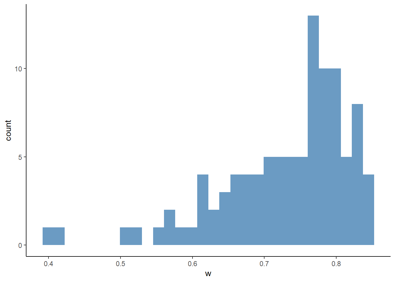

Write a function compute_winning_bids_first(valuation, reserve, alpha, beta) that returns only the winning bids from each first-price auction. It will call compute_bids_first inside the function. It does not return anything when no bidder bids above the reserve price.

# compute winning bids from first-price auctions
df_first_w <-
  compute_winning_bids_first(
    valuation = valuation,
    reserve = reserve,
    alpha = alpha,
    beta = beta
    )
df_first_w

## # A tibble: 100 × 5
##        t     n     m     r     w
##    <int> <int> <int> <dbl> <dbl>
##  1     1     8     8   0.2 0.731
##  2     2    10    10   0.2 0.638
##  3     3     7     5   0.2 0.525
##  4     4    11     8   0.2 0.818
##  5     5    14    12   0.2 0.842
##  6     6    12    11   0.2 0.833
##  7     7    11     9   0.2 0.772
##  8     8     9     9   0.2 0.753
##  9     9    14    14   0.2 0.849
## 10    10    11     9   0.2 0.803
## # ℹ 90 more rows

ggplot(
  df_first_w, 
  aes(x = w)
  ) + 
  geom_histogram(
    fill = "steelblue", 
    alpha = 0.8
    ) + 
  theme_classic()

## `stat_bin()` using `bins = 30`. Pick better value with
## `binwidth`.

19.2 Estimate the parameters

We first estimate the parameters from the winning bids data of second-price auctions. We estimate the parameters by maximizing a log-likelihood.

\[ l(\alpha, \beta) := \frac{1}{T} \sum_{t = 1}^T \ln\frac{h_t(w_t)^{1\{m_t > 1\}} \mathbb{P}\{m_t = 1\}^{1\{m_t = 1\}}}{1 - \mathbb{P}\{m_t = 0\}}, \] where: \[ \mathbb{P}\{m_t = 0\} := F_X(r_t)^{n_t}, \] \[ \mathbb{P}\{m_t = 1\} := n_t F_X(r_t; \alpha, \beta)^{n_t - 1} [1 - F_X(r_t; \alpha, \beta)]. \]

\[ h_t(w_t) := n_t (n_t - 1) F_X(w_t; \alpha, \beta)^{n_t - 2} [1 - F_X(w_t; \alpha, \beta)] f_X(w_t; \alpha, \beta). \]

Write a function compute_p_second_w(w, r, m, n, alpha, beta) that computes \(\mathbb{P}\{m_t = 1\}\) if \(m_t = 1\) and \(h_t(w_t)\) if \(m_t > 1\).

# compute probability density for winning bids from a second-price auction
w <- df_second_w[1, ]$w
r <- df_second_w[1, ]$r
m <- df_second_w[1, ]$m
n <- df_second_w[1, ]$n
compute_p_second_w(
  w = w, 
  r = r, 
  m = m,
  n = n,
  alpha = alpha,
  beta = beta
  )

## [1] 2.752949

Write a function compute_m0(r, n, alpha, beta) that computes \(\mathbb{P}\{m_t = 0\}\).

# compute non-participation probability
compute_m0(
  r = r, 
  n = n, 
  alpha = alpha, 
  beta = beta
  )

## [1] 1.368569e-08

Write a function compute_loglikelihood_second_price_w(theta, df_second_w) that computes the log-likelihood for a second-price auction winning bid data.

# compute log-likelihood for winning bids from second-price auctions
theta <- 
  c(
    alpha, 
    beta
    )
compute_loglikelihood_second_price_w(
  theta = theta, 
  df_second_w = df_second_w
  )

## [1] 0.9849261

Compare the value of objective function around the true parameters.

# label
label <- 
  c(
    "\\alpha",
    "\\beta"
    )
label <- 
  paste(
    "$", 
    label, 
    "$",
    sep = ""
    )
# compute the graph
graph <- 
  foreach (
    i = 1:length(theta)
    ) %do% {
  theta_i <- theta[i]
  theta_i_list <- 
    theta_i * seq(
      0.8,
      1.2, 
      by = 0.05
      )
  objective_i <-
    foreach (
      j = 1:length(theta_i_list),
      .packages = c(
                    "EmpiricalIO",
                    "foreach",
                    "magrittr"
                   ),
      .combine = "rbind"
      ) %dopar% {
               theta_ij <- theta_i_list[j]
               theta_j <- theta
               theta_j[i] <- theta_ij
               objective_ij <- 
                 compute_loglikelihood_second_price_w(
                   theta_j, 
                   df_second_w
                   )
               return(objective_ij)
             }
  df_graph <- 
    data.frame(
      x = as.numeric(theta_i_list), 
      y = as.numeric(objective_i)
      )
  g <- 
    ggplot(
      data = df_graph, 
      aes(
        x = x,
        y = y
        )
      ) +
    geom_point() +
    geom_vline(
      xintercept = theta_i,
      linetype = "dotted"
      ) +
    ylab("objective function") + 
    xlab(TeX(label[i])) + 
    theme_classic()
  return(g)
}
saveRDS(
  graph, 
  file = "lecture/data/a9/second_parametric_graph.rds" %>% here::here()
)

graph <- 
  readRDS(
    file = "lecture/data/a9/second_parametric_graph.rds" %>% here::here()
  )
graph

## [[1]]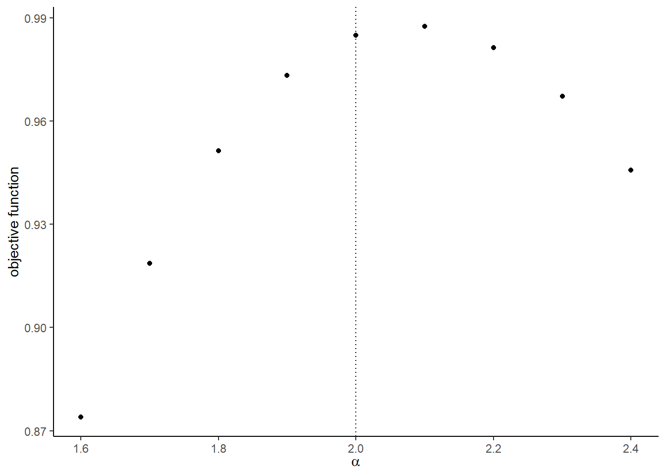

## 
## [[2]]

Estimate the parameters by maximizing the log-likelihood.

result_second_parametric <-
  optim(
    par = theta,
    fn = compute_loglikelihood_second_price_w,
    df_second_w = df_second_w,
    method = "L-BFGS-B",
    control = list(fnscale = -1)
  )
saveRDS(
  result_second_parametric, 
  file = "lecture/data/a9/result_second_parametric.rds" %>% here::here()
)

result_second_parametric <- 
  readRDS(
    file = "lecture/data/a9/result_second_parametric.rds" %>% here::here()
  )
result_second_parametric

## $par
## [1] 2.199238 2.078327
## 
## $value
## [1] 0.9883372
## 
## $counts
## function gradient 
##       11       11 
## 
## $convergence
## [1] 0
## 
## $message
## [1] "CONVERGENCE: REL_REDUCTION_OF_F <= FACTR*EPSMCH"

comparison <-

  data.frame(
    true = theta,
    estimate = result_second_parametric$par
  )
comparison

##   true estimate
## 1    2 2.199238
## 2    2 2.078327

Next, we estimate the parameters from the winning bids data from first-price auctions. We estimate the parameters by maximizing a log-likelihood.

Write a function inverse_bid_equation(x, b, r, alpha, beta, n) that returns \(\beta(x) - b\) for a bid \(b\). Write a function inverse_bid_first(b, r, alpha, beta, n) that is an inverse function bid_first with respect to the signal, that is, \[ \eta(b) := \beta^{-1}(b). \]

To do so, we can use a built-in function called uniroot, which solves \(x\) such that \(f(x) = 0\) for scalar \(x\). In uniroot, lower and upper are set at \(r_t\) and \(1\), respectively.

r <- df_first_w[1, "r"] %>%
  as.numeric()
n <- df_first_w[1, "n"] %>%
  as.integer()
b <- 0.5 * r + 0.5 
x <- 0.5
# compute inverse bid equation
inverse_bid_equation(
  x = x,
  b = b,
  r = r,
  alpha = alpha, 
  beta = beta,
  n = n
  )

## [1] -0.1421105

# compute inverse bid
inverse_bid_first(
  b = b, 
  r = r,
  alpha = alpha,
  beta = beta,
  n = n
  )

## [1] 0.6653238

The log-likelihood conditional on \(m_t \ge 1\) is: \[ l(\alpha, \beta) := \frac{1}{T}\sum_{t = 1}^T \log \frac{h_t(w_t)}{1 - F_X(r_t)^{n_t}}, \] where the probability density of having \(w_t\) is: \[ \begin{split} h_t(w_t) &= n_t F_X[\eta_t(w_t)]^{n_t - 1} f_X[\eta_t(w_t)] \eta_t'(w_t)\\ &= \frac{n_t F_X[\eta_t(w_t)]^{n_t}}{(n_t - 1)[\eta_t(w_t) - w_t]}, \end{split} \] where the second equation is from the first-order condition.

Write a function compute_p_first_w(w, r, alpha, beta, n) that returns \(h_t(w)\). Remark that the equilibrium bid at specific parameters is bid_first(1, r, alpha, beta, n). If the observed wining bid w is above the upper limit, the function will issue an error. Therefore, inside the function compute_p_first_w(w, r, alpha, beta, n), check if w is above bid_first(1, r, alpha, beta, n) and if so return \(10^{-6}\).

# compute probability density for a winning bid from a first-price auction
w <- 0.5
compute_p_first_w(
  w = w, 
  r = r, 
  alpha = alpha, 
  beta = beta, 
  n = n
  )

## [1] 0.2720049

upper <- 
  bid_first(
  x = 1, 
  r = r, 
  alpha = alpha, 
  beta = beta, 
  n = n
  )
compute_p_first_w(
  w = upper + 1, 
  r = r, 
  alpha = alpha, 
  beta = beta, 
  n = n
  )

## [1] 1e-06

Write a function compute_loglikelihood_first_price_w(theta, df_first_w) that computes the log-likelihood for a first-price auction winning bid data.

# compute log-likelihood for winning bids for first-price auctions
compute_loglikelihood_first_price_w(
  theta = theta, 
  df_first_w = df_first_w
  )

## [1] 1.597414

Compare the value of the objective function around the true parameters.

theta <- 
  c(
    alpha,
    beta
    )
# label
label <- 
  c(
    "\\alpha",
    "\\beta"
    )
label <- 
  paste(
    "$",
    label,
    "$", 
    sep = ""
    )
# compute the graph
graph <- 
  foreach (
    i = 1:length(theta)
    ) %do% {
  theta_i <- theta[i]
  theta_i_list <- 
    theta_i * seq(
      0.8,
      1.2,
      by = 0.05
      )
  objective_i <-
    foreach (
      j = 1:length(theta_i_list),
      .packages = c(
        "EmpiricalIO",
        "foreach",
        "magrittr"
        ),
      .combine = "rbind"
      ) %dopar% {
               theta_ij <- theta_i_list[j]
               theta_j <- theta
               theta_j[i] <- theta_ij
               objective_ij <- 
                 compute_loglikelihood_first_price_w(
                   theta_j,
                   df_first_w
                   )
               return(objective_ij)
             }
  df_graph <- 
    data.frame(
      x = as.numeric(theta_i_list), 
      y = as.numeric(objective_i)
      )
  g <-
    ggplot(
      data = df_graph,
      aes(
        x = x,
        y = y
        )
      ) +
    geom_point() +
    geom_vline(
      xintercept = theta_i, 
      linetype = "dotted"
      ) +
    ylab("objective function") + 
    xlab(TeX(label[i])) + 
    theme_classic()
  return(g)
}
saveRDS(
  graph,
  file = "lecture/data/a9/first_parametric_graph.rds" %>% here::here()
)

graph <- 
  readRDS(
    file = "lecture/data/a9/first_parametric_graph.rds" %>% here::here()
  )
graph

## [[1]]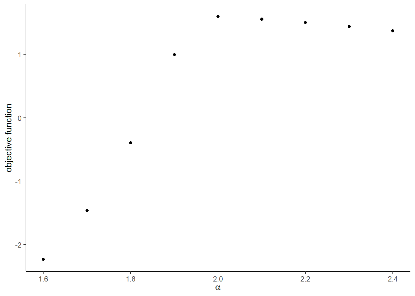

## 
## [[2]]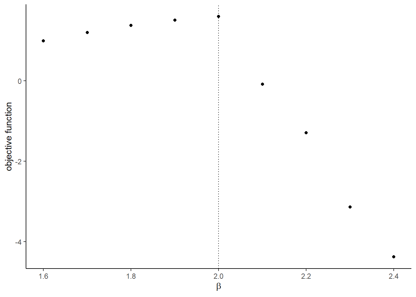

Estimate the parameters by maximizing the log-likelihood. Set the lower bounds at zero. Use the Nelder-Mead method. Otherwise the parameter search can go to extreme values because of the discontinuity at the point where the upper limit is below the observed bid.

result_first_parametric <-
  optim(
    par = theta,
    fn = compute_loglikelihood_first_price_w,
    df_first_w = df_first_w,
    method = "Nelder-Mead",
    control = list(fnscale = -1)
  )
saveRDS(
  result_first_parametric,
  file = "lecture/data/a9/result_first_parametric.rds" %>% here::here()
)

result_first_parametric <- 
  readRDS(
    file = "lecture/data/a9/result_first_parametric.rds" %>% here::here()
  )
result_first_parametric

## $par
## [1] 1.977676 2.004715
## 
## $value
## [1] 1.607161
## 
## $counts
## function gradient 
##       91       NA 
## 
## $convergence
## [1] 0
## 
## $message
## NULL

comparison <-

  data.frame(
    true = theta,
    estimate = result_first_parametric$par
  )
comparison

##   true estimate
## 1    2 1.977676
## 2    2 2.004715

Finally, we non-parametrically estimate the distribution of the valuation using bid data from first-price auctions df_first.

Write a function F_b(b) that returns an empirical cumulative distribution at b. This can be obtained by using a function ecdf. Also, write a function f_b(b) that returns an empirical probability density at b. This can be obtained by combining functions approxfun and density.

# cumulative distribution
ggplot(
  df_first, 
  aes(x = b)
  ) + 
  stat_ecdf(color = "steelblue") +
  xlab("bid") + 
  ylab("cumulative distribution") + 
  theme_classic()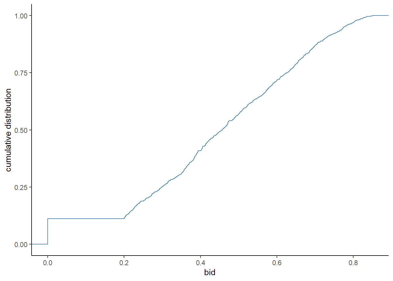

F_b <- ecdf(df_first$b)
F_b(0.4)

## [1] 0.4104628

F_b(0.6)

## [1] 0.7173038

# probability density
ggplot(
  df_first, 
  aes(x = b)
  ) + 
  geom_density(fill = "steelblue") + 
  theme_classic()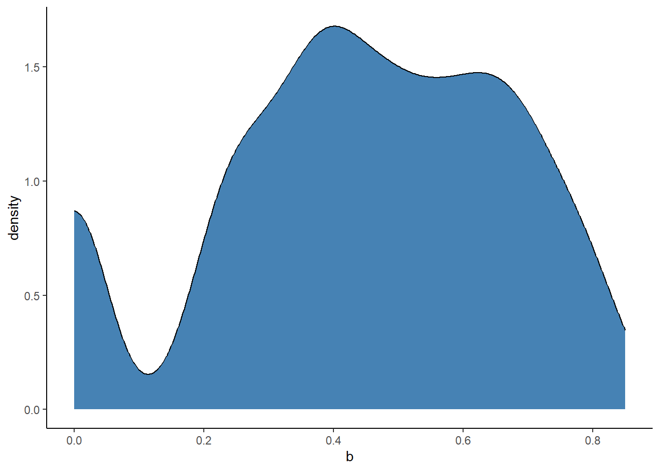

f_b <- approxfun(density(df_first$b))
f_b(0.4)

## [1] 1.678718

f_b(0.6)

## [1] 1.468564

The equilibrium distribution and density of the highest rival’s bid are: \[ H_b(b) := F_b(b)^{n - 1}, \] \[ h_b(b) := (n - 1) f_b(b) F_b(b)^{n - 2}. \]

Write a function H_b(b, n, F_b) and h_b(b, n, F_b, f_b) that return the equilibrium distribution and density of the highest rival’s bid at point b.

H_b(
  b = 0.4,
  n = n,
  F_b = F_b
  )

## [1] 0.001962983

h_b(
  b = 0.4,
  n = n,
  F_b = F_b, 
  f_b
  )

## [1] 0.0561977

When a bidder bids \(b\), the implied valuation of her is: \[ x = b + \frac{H_b(b)}{h_b(b)}. \]

Write a function compute_implied_valuation(b, n, r) that returns the implied valuation given a bid. Let it return \(x = 0\) if \(b < r\), because we cannot know the value when the bid is below the reserve price.

r <- df_first[1, "r"]
n <- df_first[1, "n"]
compute_implied_valuation(
  b = 0.4,
  n = n, 
  r = r, 
  F_b = F_b, 
  f_b = f_b
  )

##           n
## 1 0.4349299

Obtain the vector of implied valuations from the vector of bids and draw the empirical cumulative distribution. Overlay it with the true empirical cumulative distribution of the valuations.

valuation_implied <- 
  df_first %>%
  dplyr::rowwise() %>%
  dplyr::mutate(
    x = compute_implied_valuation(
      b, 
      n,
      r,
      F_b, 
      f_b
      )
    ) %>%
  dplyr::ungroup() %>%
  dplyr::select(x) %>%
  dplyr::mutate(type = "estimate")
valuation_true <- 
  valuation %>%
  dplyr::select(x) %>%
  dplyr::mutate(type = "true")
valuation_plot <- 
  rbind(
    valuation_true,
    valuation_implied
    )
ggplot(
  valuation_plot,
  aes(
    x = x, 
    color = type
    )
  ) + 
  stat_ecdf() + 
  theme_classic()